Spinal Sonography and Considerations for Ultrasound-Guided Central Neuraxial Blockade
Wing Hong Kwok and Manoj Karmakar
Introduction
Ultrasound scanning (US) can offer several advantages when used to guide placement of the needle for centroneuraxial blocks (CNBs). It is noninvasive, safe, simple to use, can be performed expeditiously, provides real-time images, is devoid from adverse effects, and it may be beneficial in patients with abnormal or variant spinal anatomy. When used for chronic pain interventions, US also eliminates or reduces exposure to radiation. In expert hands, the use of US for epidural needle insertion was shown to reduce the number of puncture attempts,1–4 improve the success rate of epidural access on the first attempt,2 reduce the need to puncture multiple levels,2–4 and improve patient comfort during the procedure.3 These advantages led the National Institute of Clinical Excellence (NICE) in the United Kingdom to recommend the routine use of ultrasound for epidural blocks.5 Incorporating these recommendations into clinical practice, however, has met significant obstacles. As one example, a recent survey of anesthesiologists in the United Kingdom showed that >90% of respondents were not trained in the use of US to image the epidural space.6 In this chapter, we describe techniques of US imaging of the spine, the relevant sonoanatomy, and practical considerations for using US-guided CNB and nerve blocks close to the centroneuroaxis.
Historical Background
Bogin and Stulin were probably the first to report using US for central neuraxial interventional procedures.7 In 1971, they described using US to perform lumbar puncture.7 Porter and colleagues, in 1978, used US to image the lumbar spine and measure the diameter of the spinal canal in diagnostic radiology.8 Cork and colleagues were the first group of anesthesiologists to use US to locate the landmarks relevant for epidural anesthesia.9 Thereafter, US was used mostly to preview the spinal anatomy and measure the distances from the skin to the lamina and epidural space before epidural puncture.10,11 More recently, Grau and coworkers, from Heidelberg in Germany, conducted a series of studies, significantly contributing to the current understanding of spinal sonography.1–4,12–15 These investigators described a two-operator technique consisting of real-time US visualization of neuraxial space using a paramedian sagittal axis and insertion of the needle through the midline to accomplish a combined spinal-epidural block.4 The quality of the US image at the time, however, was substantially inferior to that of today’s equipment, thus hindering acceptance and further research in this area. Recent improvements in US technology and image clarity have allowed for much greater clarity during imaging of the spine and neuraxial structures.16,17
Ultrasound Imaging of the Spine
Basic Considerations
Because the spine is located at a depth, US imaging of the spine typically requires the use of low-frequency ultrasound (5-2 MHz) and curved array transducers. Low-frequency US provides good penetration but unfortunately, it lacks the spatial resolution at the depth (5–7 cm) at which the neuraxial structures are located. The osseous framework of the spine, which envelops the neuraxial structures, reflects much of the incident US signal before it reaches the spinal canal, presenting additional challenges in obtaining good quality images. Recent improvements in US technology, the greater image processing capabilities of US machines, the availability of compound imaging, and the development of new scanning protocols have improved the ability to image the neuraxial space significantly. As a result, today it is possible to reasonably accurately delineate the neuraxial anatomy relevant for CNB. Also of note is that technology once only available in the high-end, cart-based U.S. systems is now available in portable US devices, making them even more practical for spinal sonography and US-guided CNB applications.
Ultrasound Scan Planes
Although anatomic planes have already been described elsewhere in this text, the importance of understanding them for imaging of the neuraxial space dictates another, more detailed review. There are three anatomical planes: median, transverse, and coronal (Figure 44-1). The median plane is a longitudinal plane that passes through the midline bisecting the body into equal right and left halves. The sagittal plane is a longitudinal plane that is parallel to the median plane and perpendicular to the ground. Therefore, the median plane also can be defined as the sagittal plane that is exactly in the middle of the body (median sagittal plane). The transverse plane, also known as the axial or horizontal plane, is parallel to the ground. The coronal plane, also known as the frontal plane, is perpendicular to the ground. A US scan of the spine can be performed in the transverse (transverse scan) or longitudinal (sagittal scan) axis with the patient in the sitting, lateral decubitus, or prone position. The two scanning planes complement each other during a US examination of the spine. A sagittal scan can be performed through the midline (median sagittal scan) or through a paramedian (paramedian sagittal scan) plane. Grau et al suggested a paramedian sagittal plane to visualize the neuraxial structures.12 The US visibility of neuraxial structures can be further improved when the spine is imaged in the paramedian oblique sagittal. During a paramedian oblique sagittal scan (PMOSS), the transducer is positioned 2 to 3 cm lateral to the midline (paramedian) in the sagittal axis and it is also tilted slightly medially, that is, toward the midline (Figure 44-2). The purpose of the medial tilt is to ensure that the US signal enters the spinal canal through the widest part of the interlaminar space and not the lateral sulcus of the canal.
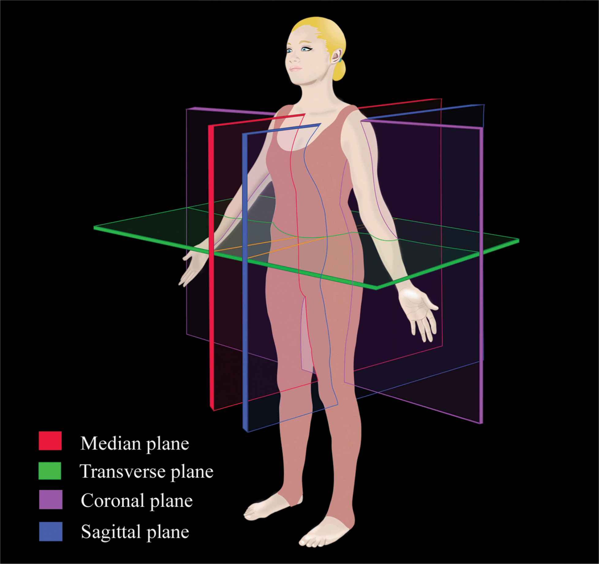
FIGURE 44-1. Anatomic planes of the body.
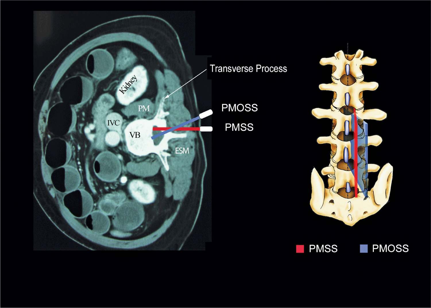
FIGURE 44-2. Paramedian sagittal scan (PMSS) of the lumbar spine. The PMSS is represented by the red color and the paramedian oblique sagittal axis of scan (PMOSS) is represented by the blue color. Note how the plane of imaging during a PMOSS is tilted slightly medially. This is done to ensure that most of the ultrasound energy enters the spinal canal through the widest part of the interlaminar space. ICV, inferior vena cava; VB, vertebral body; PM, psoas muscle; ESM, erector spinae muscle.
Sonoanatomy of the Spine
Detailed knowledge of the vertebral anatomy is essential to understand the sonoanatomy of the spine. Unfortunately, cross-sectional anatomy texts describe the anatomy of the spine in traditional orthogonal planes, that is, the transverse, sagittal, and coronal planes. This often results in difficulty interpreting the spinal sonoanatomy because US imaging is generally performed in an arbitrary or intermediary plane by tilting, sliding, and rotating the transducer. Moreover, currently there are limited data on spinal sonography or on how to interpret US images of the spine.
Several anatomic models recently became available that can be used to learn musculoskeletal US imaging techniques (human volunteers), the sonoanatomy relevant for peripheral nerve blocks (human volunteers or cadavers), and the required interventional skills (tissue mimicking phantoms, fresh cadavers). However, few models or tools are available to learn and practice spinal sonoanatomy or the interventional skills required for US-guided CNB. Karmakar and colleagues recently described the use of a “water-based spine phantom” (Figure 44-3A) to study the osseous anatomy of the lumbosacral spine16,18 and a “pig carcass phantom” model19 (Figure 44-4A) to practice the hand-eye coordination skills required to perform US-guided CNB.19 Computer-generated anatomic reconstruction from the Visible Human Project data set that corresponds to the US scan planes is another useful way of studying the sonoanatomy of the spine. Multiplanar three-dimensional (3D) reconstruction from a high-resolution 3D computed tomography (CT) data set of the spine can be used to study and validate the sonographic appearance of the various osseous elements of the spine (Figure 44-5).
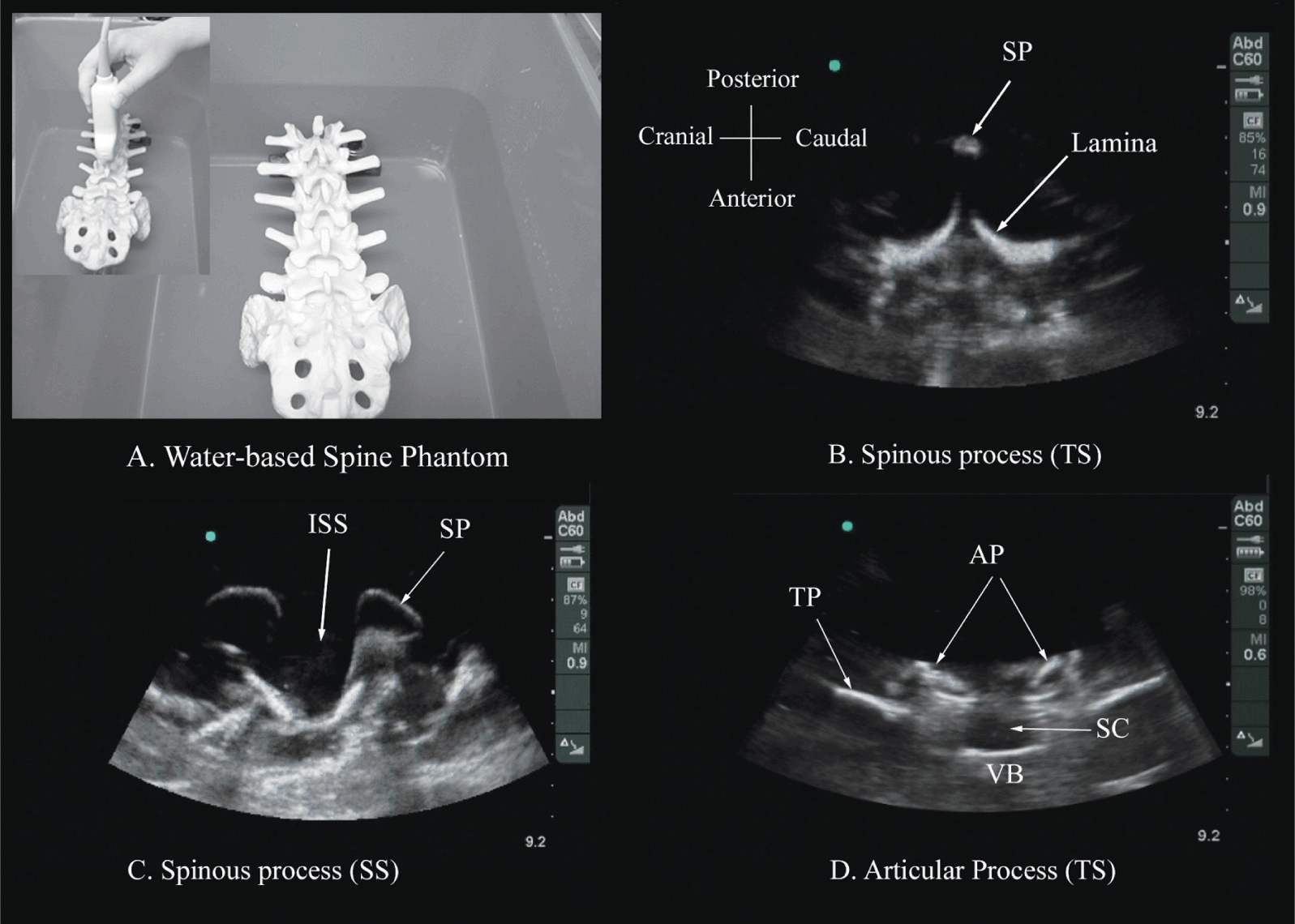
FIGURE 44-3. (A) The water-based spine phantom and sonograms of the spinous process in the (B) transverse and (C) midsagittal or median axes, and (D) a scan through the interspinous space. SP, spinous process; ISS, interspinous space; TP, transverse process; AP, articular process; SC, spinal canal; VB, vertebral body; TS, transverse scan; SS, sagittal scan.
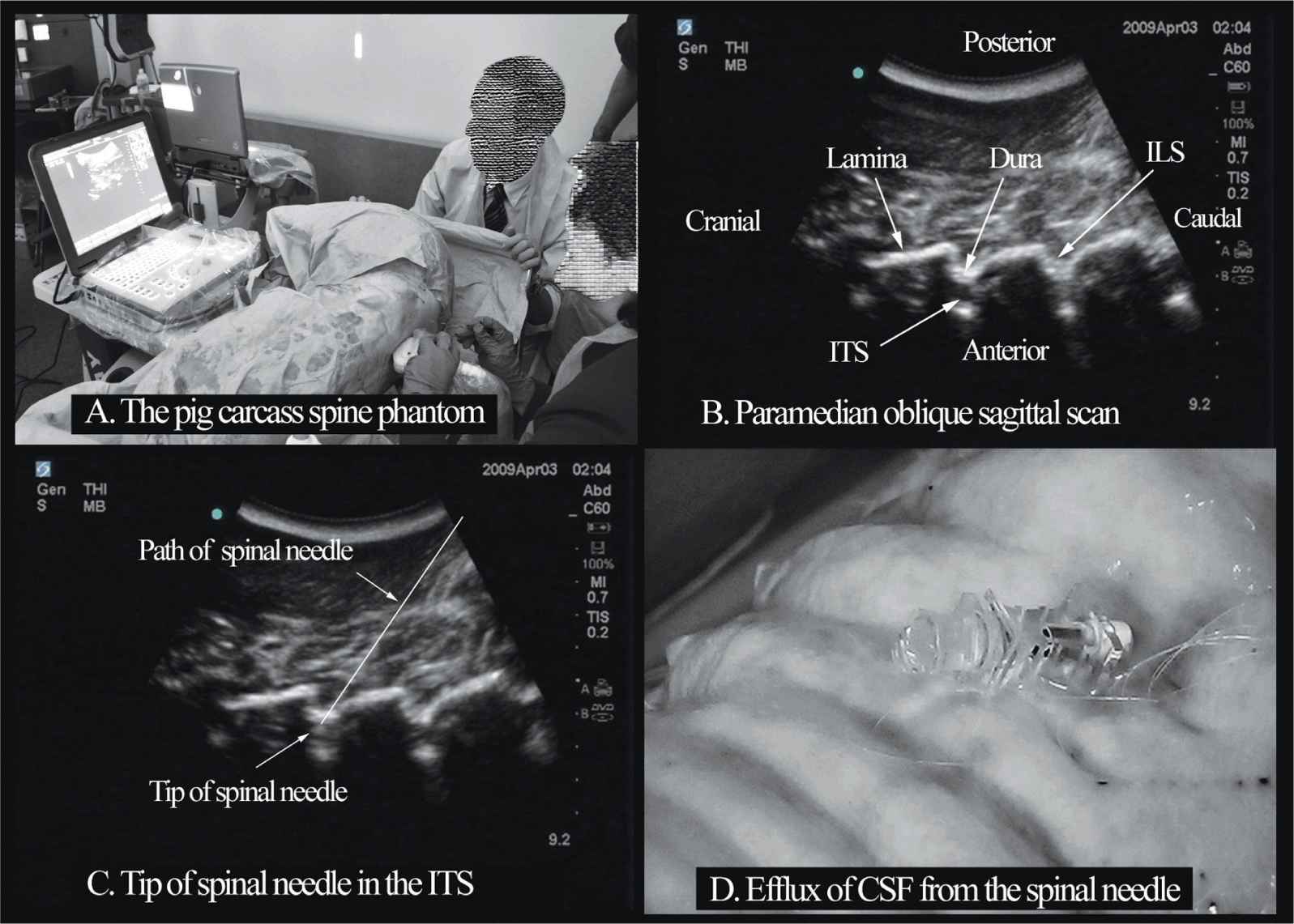
FIGURE 44-4. The “Pig carcass spine phantom” (A) being used to practice central neuraxial blocks at a workshop, (B) paramedian oblique sagittal sonogram of the lumbar spine, (C) sonogram showing the tip of a spinal needle in the ITS (intrathecal space), (D) picture showing the efflux of cerebrospinal fluid (CSF) from the hub of a spinal needle that has been inserted into the ITS. ILS, interlaminar space.
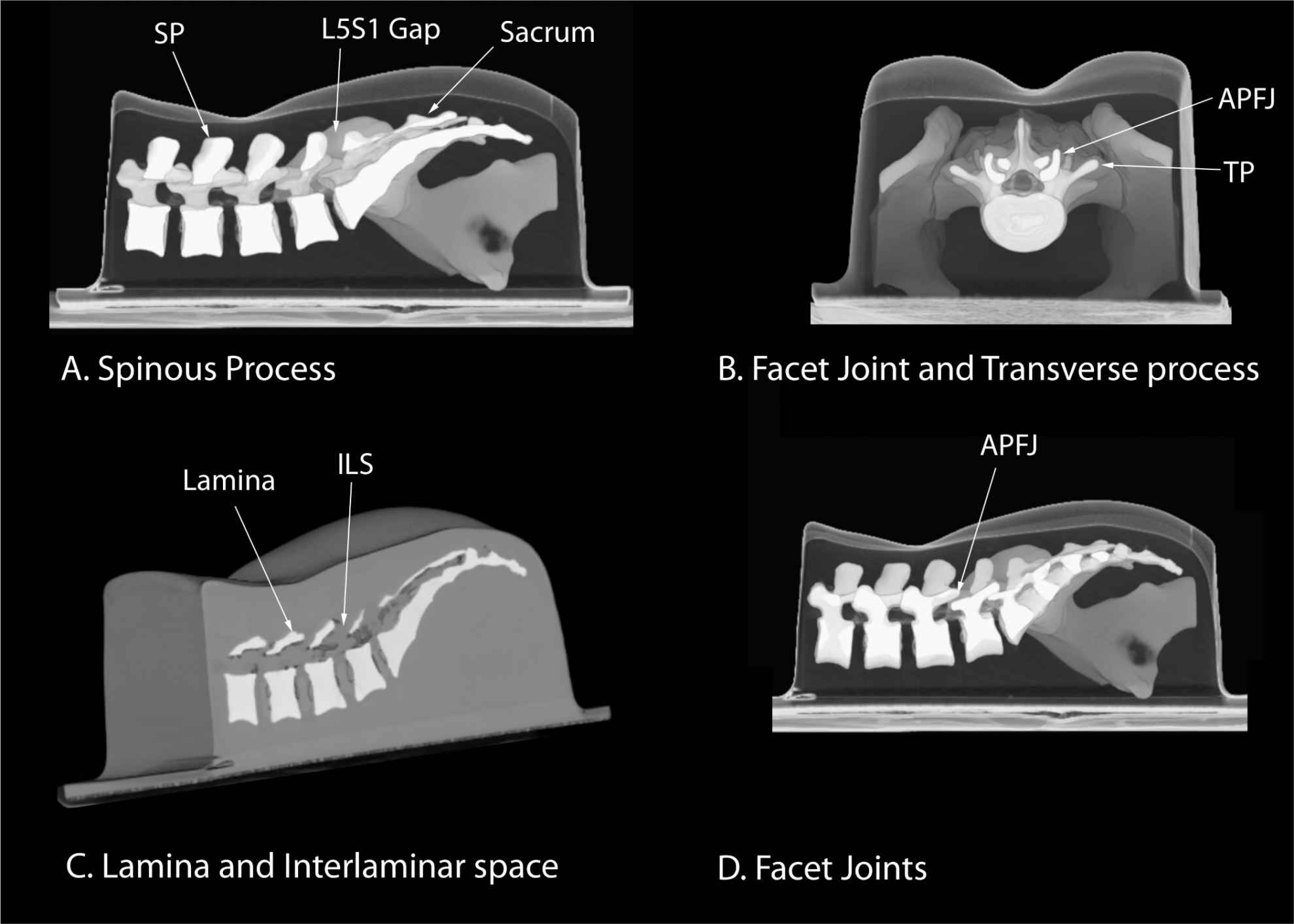
FIGURE 44-5. Three-dimensional reconstruction of high-resolution computed tomography scan data set from a lumbar training phantom (CIRS Model 034, CIRS Inc., Norfolk, VA, USA). (A) Median sagittal scan of the spinous process (SP), (B) transverse interspinous view of the articular process (AP), transverse process (TP), and facet joint (FJ), (C) paramedian oblique sagittal scan showing the lamina and interlaminar space (ILS), and (D) paramedian sagittal scan at the level of the articular processes. ISS, interspinous space.
Water-Based Spine Phantom
The water-based spine phantom18 is based on a model described previously by Greher and colleagues to study the osseous anatomy of relevance to US-guided lumbar facet nerve block.20 The model is prepared by immersing a commercially available lumbosacral spine model in a water bath. A low-frequency curved array transducer submerged into water is used to scan in the transverse and sagittal axes (Figure 44-3A). Each osseous element of the spine produces a “characteristic” sonographic pattern. The ability to recognize these sonographic patterns is an important step toward understanding the sonoanatomy of the spine. Representative US images of the spinous process, lamina, articular processes, and the transverse process from the water-based spine phantom are presented in Figures 44-3 and 44-6. The advantage of this water-based spine phantom is that water produces an anechoic (black) background against which the hyperechoic reflections from the bone are clearly visualized. The water-based spine phantom allows a see-through real-time visual validation of the sonographic appearance of a given osseous element by performing the scan with a marker (e.g., a needle) in contact with it (Figure 44-6A). The described model is also inexpensive, easily prepared, requires little time to set up, and can be used repeatedly without deteriorating or decomposing, as animal tissue-based phantoms do.
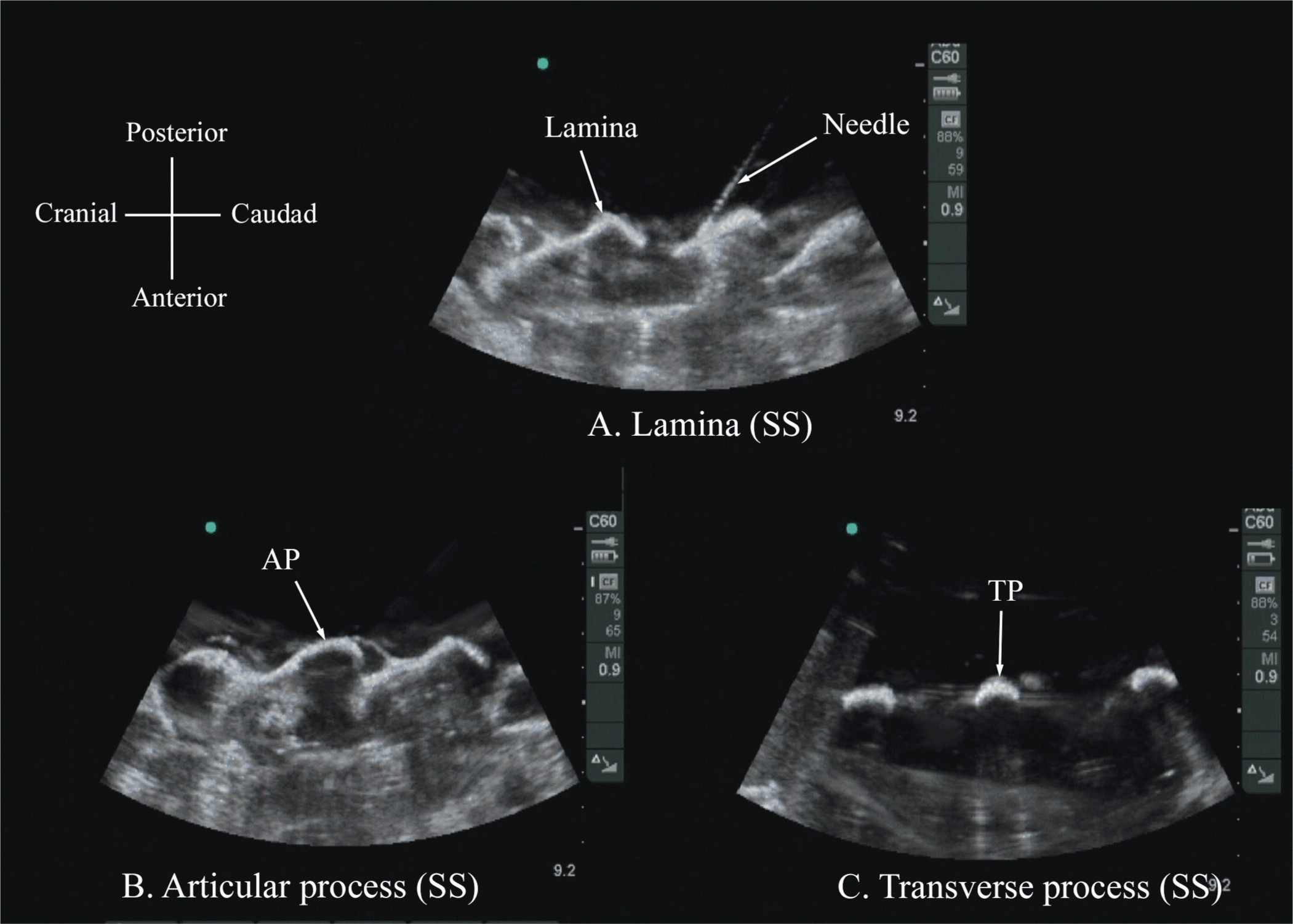
FIGURE 44-6. Paramedian sagittal sonogram of the (A) lamina, (B) articular process, and (C) transverse process from the water-based spine phantom. Note the needle in contact with the lamina in (A), a method that was used to validate the sonographic appearance of the osseous elements in the phantom.
Ultrasound Imaging of the Lumbar Spine
Sagittal Scan
The patient is positioned in the sitting, lateral, or prone position with the lumbosacral spine maximally flexed. The transducer is placed 1 to 2 cm lateral to the spinous process (i.e., in the paramedian sagittal plane) at the lower back with its orientation marker directed cranially. A slight tilt medially during the scan is assumed to insonate in a paramedian oblique sagittal plane. First, the sacrum is identified as a flat hyperechoic structure with a large acoustic shadow anteriorly (Figure 44-7). When the transducer is slid in a cranial direction, a gap is seen between the sacrum and the lamina of the L5 vertebra, which is the L5-S1 interlaminar space, also referred to as the L5-S1gap (Figure 44-7).16,17,21 The L3-4 and L4-5 interlaminar spaces can now be located by counting upward (Figure 44-8).16,17 The erector spinae muscles are hypoechoic and lie superficial to the laminae. The lamina appears hyperechoic and is the first osseous structure visualized (Figure 44-8). Because bone impedes the penetration of US, there is an acoustic shadow anterior to each lamina. The sonographic appearance of the lamina produces a pattern that resembles the head and neck of a horse, which Karmakar and colleagues referred to as the “horse head sign” (Figures 44-5C, 44-6A, and 44-8).16 The interlaminar space is the gap between the adjoining lamina and is the “acoustic window” through which the neuraxial structures are visualized within the spinal canal. The ligamentum flavum appears as a hyperechoic band across adjacent lamina). The posterior dura is the next hyperechoic structure anterior to the ligamentum flavum, and the epidural space is the hypoechoic area (a few millimeters wide) between the ligamentum flavum and the posterior dura. The thecal sac with the cerebrospinal fluid is the anechoic space anterior to the posterior dura (Figure 44-8). The cauda equina, which is located within the thecal sac, often is seen as multiple horizontal, hyperechoic shadows within the anechoic thecal sac. Pulsations of the cauda equina are identified in some patients.16,17 The anterior dura also is hyperechoic, but it is not always easy to differentiate it from the posterior longitudinal ligament and the vertebral body because they are of similar echogenicity (isoechoic) and especially closely related. Often, what results is a single, composite, hyperechoic reflection anteriorly that we refer to as the “anterior complex” (Figure 44-8).16,17 If the transducer slides medially, that is, to the median sagittal plane, the tips of the spinous processes of the L3-L5 vertebra, which appear as crescent-shaped structures, are seen (Figures 44-3C, 44-5A, and 44-9).16 The acoustic window between the spinous processes in the median plane is narrow and may prevent clear visualization of the neuraxial structures within the spinal canal. In contrast, if the transducer is moved slightly laterally from the paramedian sagittal plane at the level of the lamina, the articular processes of the vertebra are seen. The articular processes appear as one continuous, hyperechoic wavy line with no intervening gaps (Figures 44-5D, 44-6B, and 44-10), as seen at the level of the lamina.16 The articular processes in a sagittal sonogram produce a sonographic pattern that resembles multiple camel humps, which are referred to as the “camel hump sign” (Figures 44-6B and 44-10). A sagittal scan lateral to the articular processes brings the transverse processes of the L3-L5 vertebrae into view. The transverse processes are recognized by their crescent-shaped hyperechoic reflections with their concavity facing anteriorly and an acoustic shadow anterior to them (Figures 44-6C and 44-11).22 This produces a sonographic pattern that we refer to as the “trident sign” because of its resemblance to the trident (Latin tridens or tridentis) that is often associated with Poseidon, the god of the sea in Greek mythology, and the Trishula of the Hindu god Shiva (Figure 44-11).22
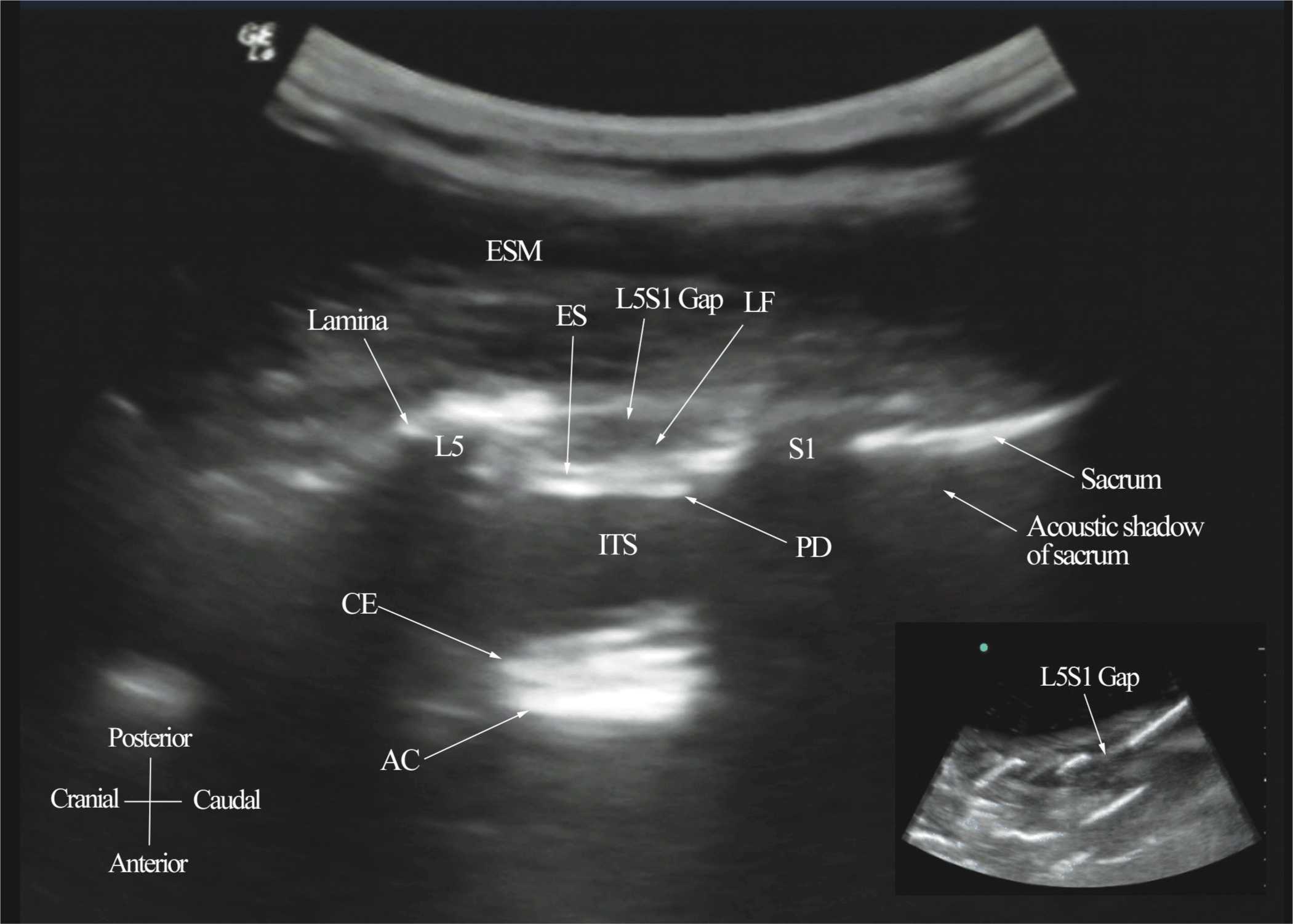
FIGURE 44-7. Paramedian sagittal sonogram of the lumbosacral junction. The posterior surface of the sacrum is identified as a flat hyperechoic structure with a large acoustic shadow anterior to it. The dip or gap between the sacrum and the lamina of L5 is the L5-S1 intervertebral space or the L5-S1 gap. ESM, erector spinae muscle; ES, epidural space; LF, ligamentum flavum; PD, posterior dura; ITS, intrathecal space; CE, cauda equina; and AC, anterior complex.
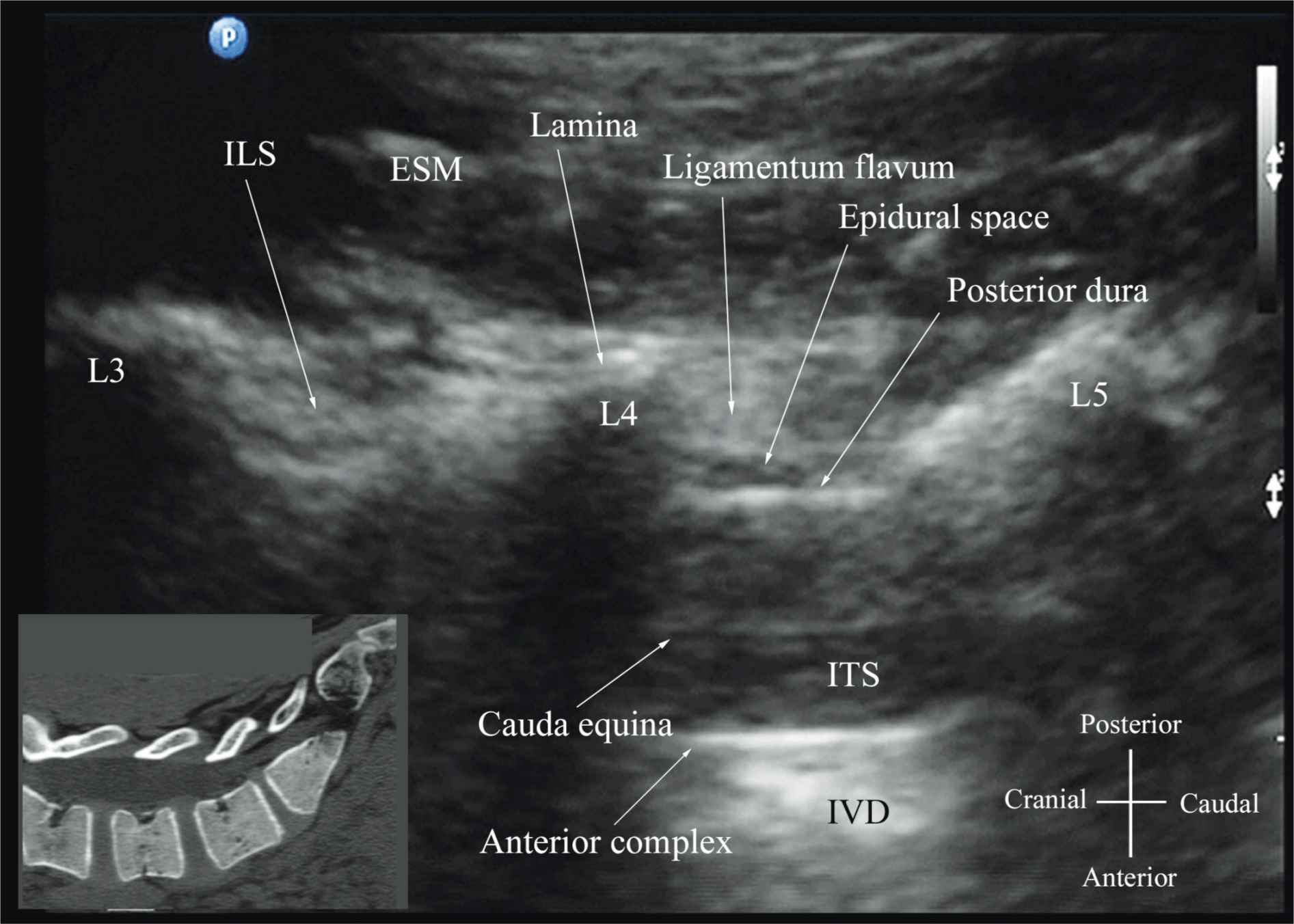
FIGURE 44-8. Paramedian oblique sagittal sonogram of the lumbar spine at the level of the lamina showing the L3-4 and L4-5 interlaminar spaces. Note the hypoechoic epidural space (few millimeters wide) between the hyperechoic ligamentum flavum and the posterior dura. The intrathecal space is the anechoic space between the posterior dura and the anterior complex in the sonogram. The cauda equina nerve fibers are also seen as hyperechoic longitudinal structures within the thecal sac. The hyperechoic reflections seen in front of the anterior complex are from the intervertebral disc (IVD). Picture in the inset shows a corresponding computed tomography (CT) scan of the lumbosacral spine in the same anatomic plane as the ultrasound scan. The CT slice was reconstructed from a three-dimensional CT data set from the author’s archive. ESM, erector spinae muscle; ILS, interlaminar space; LF, ligamentum flavum; ES, epidural space; PD, posterior dura; CE, cauda equina; ITS, intrathecal space; AC, anterior complex; IVD, intervertebral disc; L3, lamina of L3 vertebra; L4, lamina of L4 vertebra; L5, lamina of L5 vertebra.
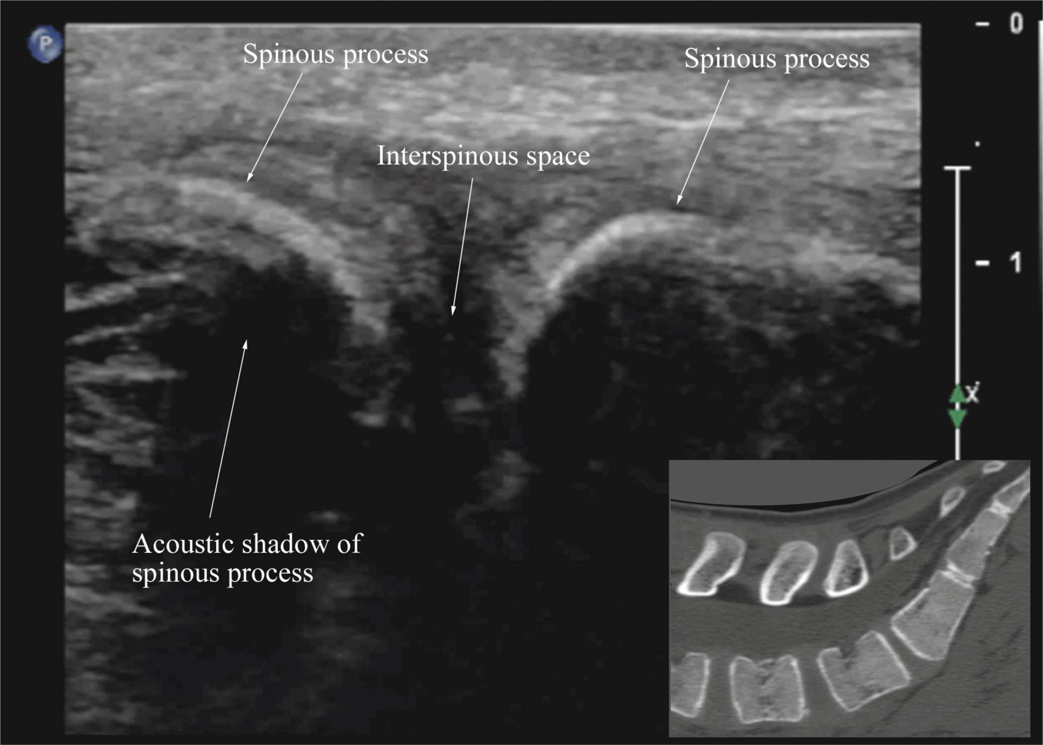
FIGURE 44-9. Median sagittal sonogram of the lumbar spine showing the crescent shaped hyperechoic reflections of the spinous processes. Note the narrow interspinous space in the midline. Picture in the inset shows a corresponding computed tomography (CT) scan of the lumbosacral spine through the median plane. The CT slice was reconstructed from a three-dimensional CT data set from the author’s archive.
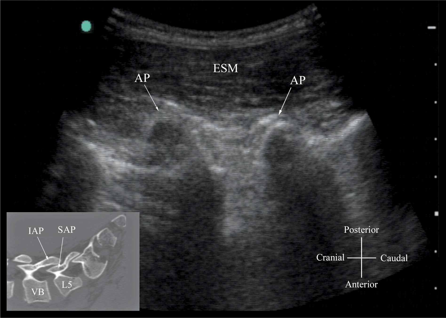
FIGURE 44-10. Paramedian sagittal sonogram of the lumbar spine at the level of the articular process (AP) of the vertebra. Note the “camel hump” appearance of the articular processes. Picture in the inset shows a corresponding computed tomography (CT) scan of the lumbosacral spine at the level of the articular processes. The CT slice was reconstructed from a three-dimensional CT data set from the author’s archive. ESM, erector spinae muscle; IAP, inferior articular process; SAP, superior articular process.
FIGURE 44-11. Paramedian sagittal sonogram of the lumbar spine at the level of the transverse processes (TPs). Note the hyperechoic reflections of the TPs with their acoustic shadow that produces the “trident sign.” The psoas muscle is seen in the acoustic window between the transverse processes and is recognized by its typical hypoechoic and striated appearance. Part of the lumbar plexus is also seen as a hyperechoic shadow in the posterior part of the psoas muscle between the transverse processes of L4 and L5 vertebra. Picture in the inset shows a corresponding computed tomography (CT) scan of the lumbosacral spine at the level of the transverse processes. The CT slice was reconstructed from a three-dimensional CT data set from the author’s archive.
Transverse Scan
For a transverse scan of the lumbar spine, the US transducer is positioned over the spinous process (transverse spinous process view) with the patient in the sitting or lateral position. On a transverse sonogram, the spinous process and the lamina on either side are seen as a hyperechoic reflection anterior to which there is a dark acoustic shadow that completely obscures the underlying spinal canal and thus the neuraxial structures (Figures 44-3B and 44-12). Therefore, this view is not suitable for imaging of the neuraxial structures but can be useful for identifying the midline when the spinous processes cannot be palpated (e.g., in obese patients). However, if the transducer is slid slightly cranially or caudally, it may be possible to perform a transverse scan through the interspinous space (transverse interspinous view) (Figures 44-3D, 44-5D, and 44-13).16,23 It is important to tilt the transducer slightly cranially or caudally to align the US beam to the interspinous space and optimize the US image. In the transverse interspinous view, the posterior dura, thecal sac, and the anterior complex can be visualized (from a posterior to anterior direction) within the spinal canal in the midline and the articular processes, and the transverse processes are visualized laterally (Figure 44-13).16,23 The ligamentum flavum is rarely visualized in the transverse interspinous view, possibly due to anisotropy caused by the arch-like attachment of the ligamentum flavum to the lamina. The epidural space is also less frequently visualized in the transverse interspinous scan than in the PMOSS. The transverse interspinous view can be used to examine for rotational deformities of the vertebra, such as in scoliosis. Normally, both the lamina and the articular processes on either side are located symmetrically (Figures 44-3D, 44-5D, and 44-13). However, if there is asymmetry, then a rotational deformity of the vertebral column24 should be suspected and the operator can anticipate a potentially difficult CNB.
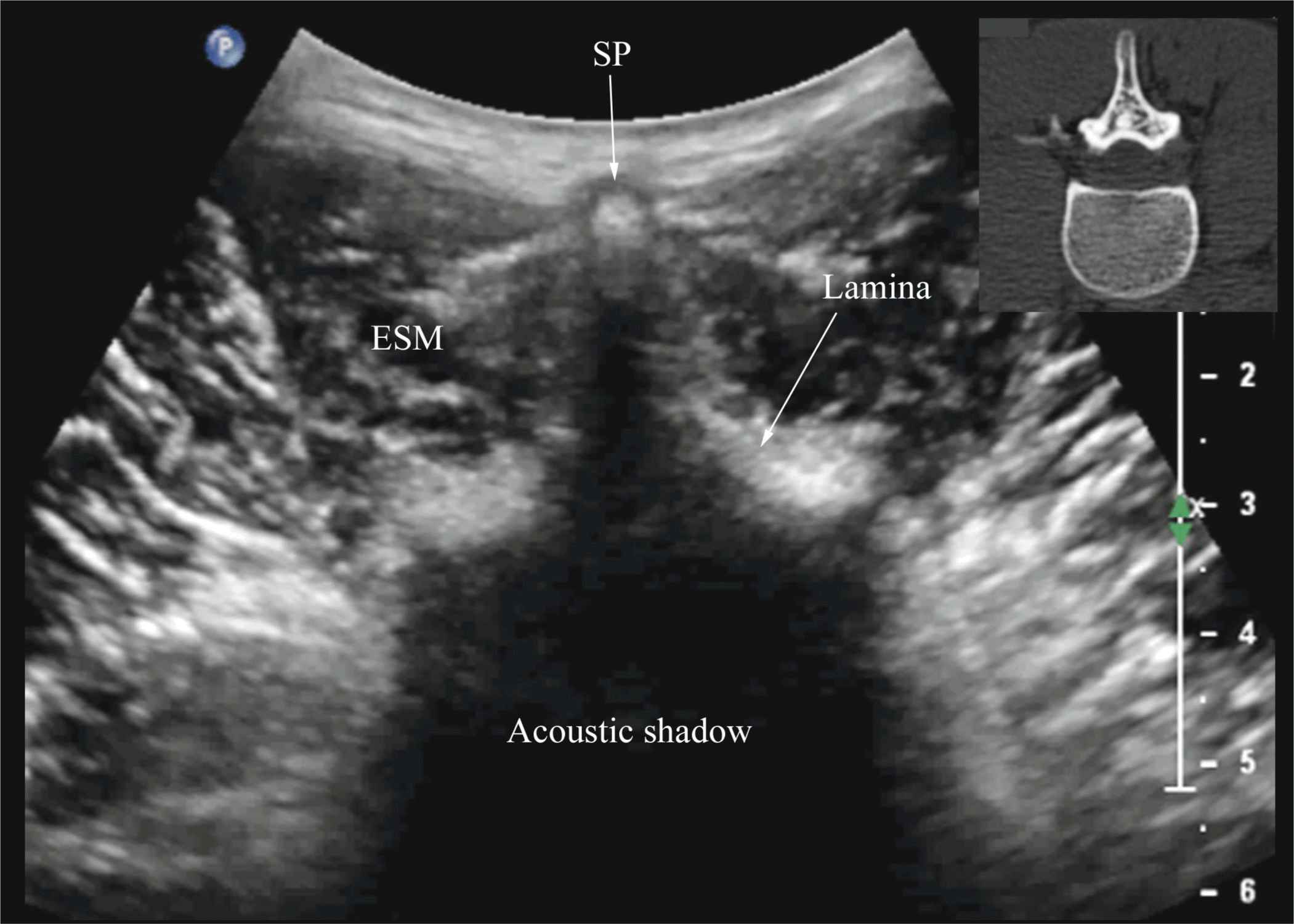
FIGURE 44-12. Transverse sonogram of the lumbar spine with the transducer positioned directly over the spinous process (i.e., transverse spinous process view). Note the acoustic shadow of the spinous process and lamina that completely obscures the spinal canal and the neuraxial structures. Picture in the inset shows a corresponding computed tomography (CT) scan of the lumbar vertebra. The CT slice was reconstructed from a three-dimensional CT data set from the author’s archive. SP, spinous process; ESM, erector spinae muscle.
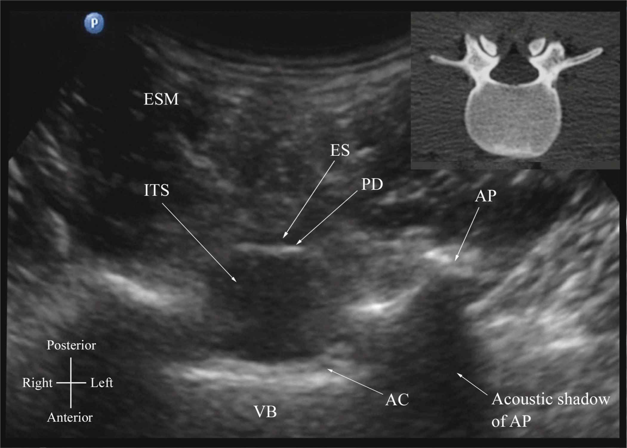
FIGURE 44-13. Transverse sonogram of the lumbar spine with the transducer positioned such that the ultrasound beam is insonated through the interspinous space (i.e., transverse interspinous view). The epidural space, posterior dura, intrathecal space, and the anterior complex are visible in the midline, and the articular process (AP) is visible laterally on either side of the midline. Note how the articular processes on either side are symmetrically located. Picture in the inset shows a corresponding computed tomography (CT) scan of the lumbar vertebra. The CT slice was reconstructed from a three-dimensional CT data set from the author’s archive. ESM, erector spinae muscle; ES, epidural space; PD, posterior dura; ITS, intrathecal space; AC, anterior complex; VB, vertebral body.
Ultrasound Imaging of the Thoracic Spine
US imaging of the thoracic spine is more challenging than imaging the lumbar spine; the ability to visualize the neuraxial structures with US may vary with the level at which the imaging is performed. Regardless of the level at which the scan is performed, the thoracic spine is probably best imaged with the patient in the sitting position. In the lower thoracic region (T9-12), the sonographic appearance of the neuraxial structures is comparable to that in the lumbar region because of comparable vertebral anatomy (Figure 44-14). However, the acute angulation of the spinous processes and the narrow interspinous and interlaminar spaces in the midthoracic region results in a narrow acoustic window with limited visibility of the underlying neuraxial anatomy (Figure 44-15). In the only published report describing US imaging of the thoracic spine, Grau and colleagues13 performed US imaging of the thoracic spine at the T5-6 level in young volunteers and correlated findings with matching magnetic resonance imaging (MRI) images. They reported that the transverse axis produced the best images of the neuraxial structures. Epidural space, however, was best visualized in the paramedian scans.13 Regardless, US was limited in being able to delineate the epidural space or the spinal cord but was better than MRI in demonstrating the posterior dura.13 The transverse interspinous view, however, is almost impossible to obtain in the midthoracic region, and therefore the transverse scan provides little useful information for CNB other than to help identify the midline. In contrast, PMOSS, despite the narrow acoustic window, provides more useful information relevant for CNB. The laminae are seen as flat hyperechoic structures with acoustic shadowing anteriorly, and the posterior dura is consistently visualized in the acoustic window (Figures 44-14 and 44-15). However, the epidural space, spinal cord, central canal, and the anterior complex are difficult to delineate in the midthoracic region (Figure 44-15).
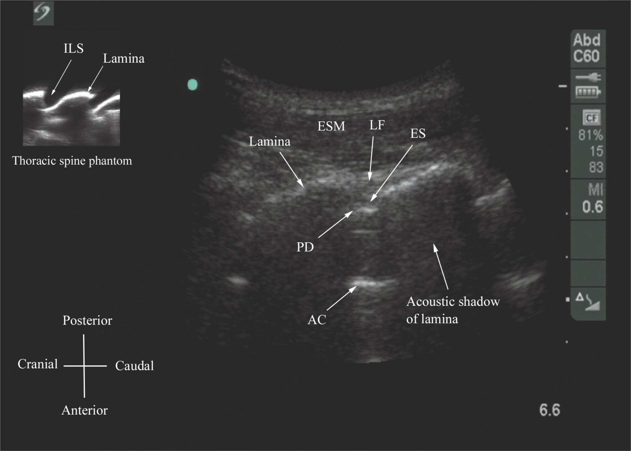
FIGURE 44-14. Paramedian oblique sagittal sonogram of the lower-thoracic spine. Note the narrow acoustic window through which the ligamentum flavum (LF), posterior dura (PD), epidural space (ES), and anterior complex (AC) are visible. Picture in the inset shows a sagittal sonogram of the thoracic spine from the water-based spine phantom. ILS, interlaminar space.
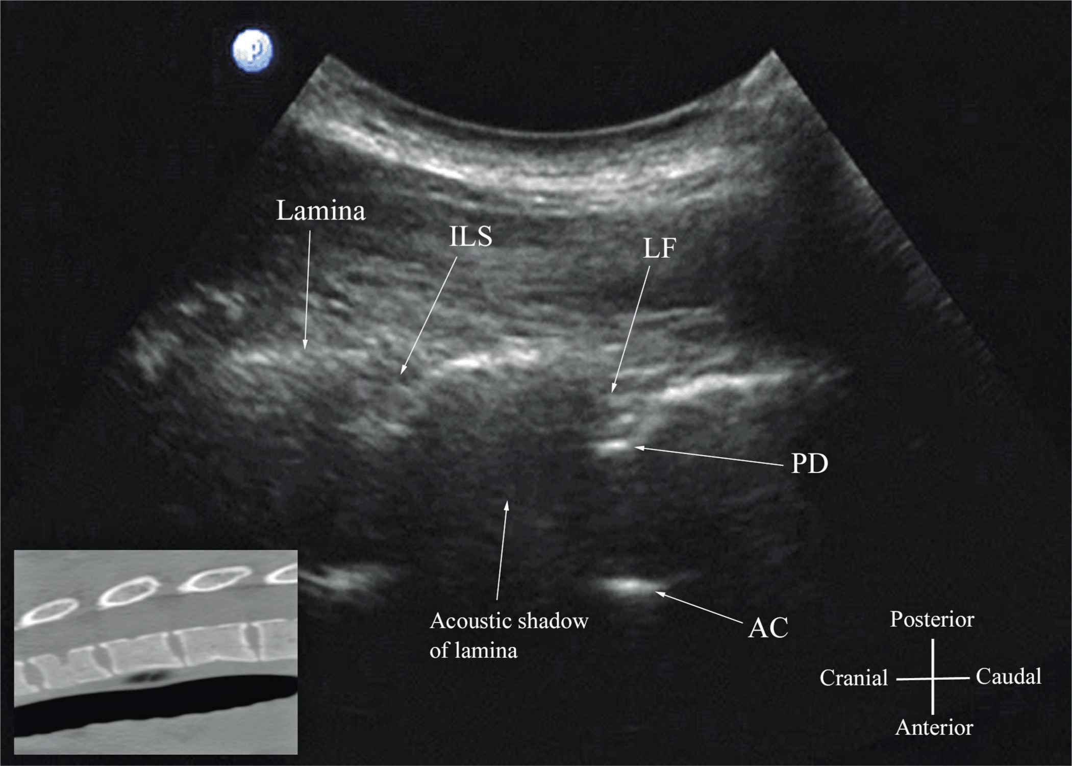
FIGURE 44-15. Paramedian oblique sagittal sonogram of the midthoracic spine. The posterior dura (PD) and the anterior complex (AC) are visible through the narrow acoustic window. Picture in the inset shows a corresponding computed tomography (CT) scan of the midthoracic spine. The CT slice was reconstructed from a three-dimensional CT data set from the author’s archive. ILS, interlaminar space; LF, ligamentum flavum.
Ultrasound Imaging of the Sacrum
Usually, US imaging of the sacrum is performed to identify the sonoanatomy relevant for a caudal epidural injection.25 Because the sacrum is a superficial structure, a high-frequency linear array transducer can be used for the scan.16,25 The patient is positioned in the lateral or prone position with a pillow under the abdomen to flex the lumbosacral spine. The caudal epidural space is the continuation of the lumbar epidural space and commonly accessed via the sacral hiatus. The sacral hiatus is located at the distal end of the sacrum, and its lateral margins are formed by the two sacral cornua covered by the sacrococcygeal ligament. On a transverse sonogram of the sacrum at the level of the sacral hiatus, the sacral cornua are seen as two hyperechoic reversed U-shaped structures, one on either side of the midline (Figure 44-16).16,25 Connecting the two sacral cornua, and deep to the skin and subcutaneous tissue, is a hyperechoic band, the sacrococcygeal ligament.16,25 Anterior to the sacrococcygeal ligament is another hyperechoic linear structure, which represents the posterior surface of the sacrum. The hypoechoic space between the sacrococcygeal ligament and the bony posterior surface of the sacrum is the caudal epidural space. The two sacral cornua and the posterior surface of the sacrum produce a pattern on the sonogram that we refer to as the “frog eye sign” because of its resemblance to the eyes of a frog (Figure 44-16).16 On a sagittal sonogram of the sacrum at the level of the sacral cornua, the sacrococcygeal ligament, the base of sacrum, and the caudal canal are also clearly visualized (Figure 44-17).16
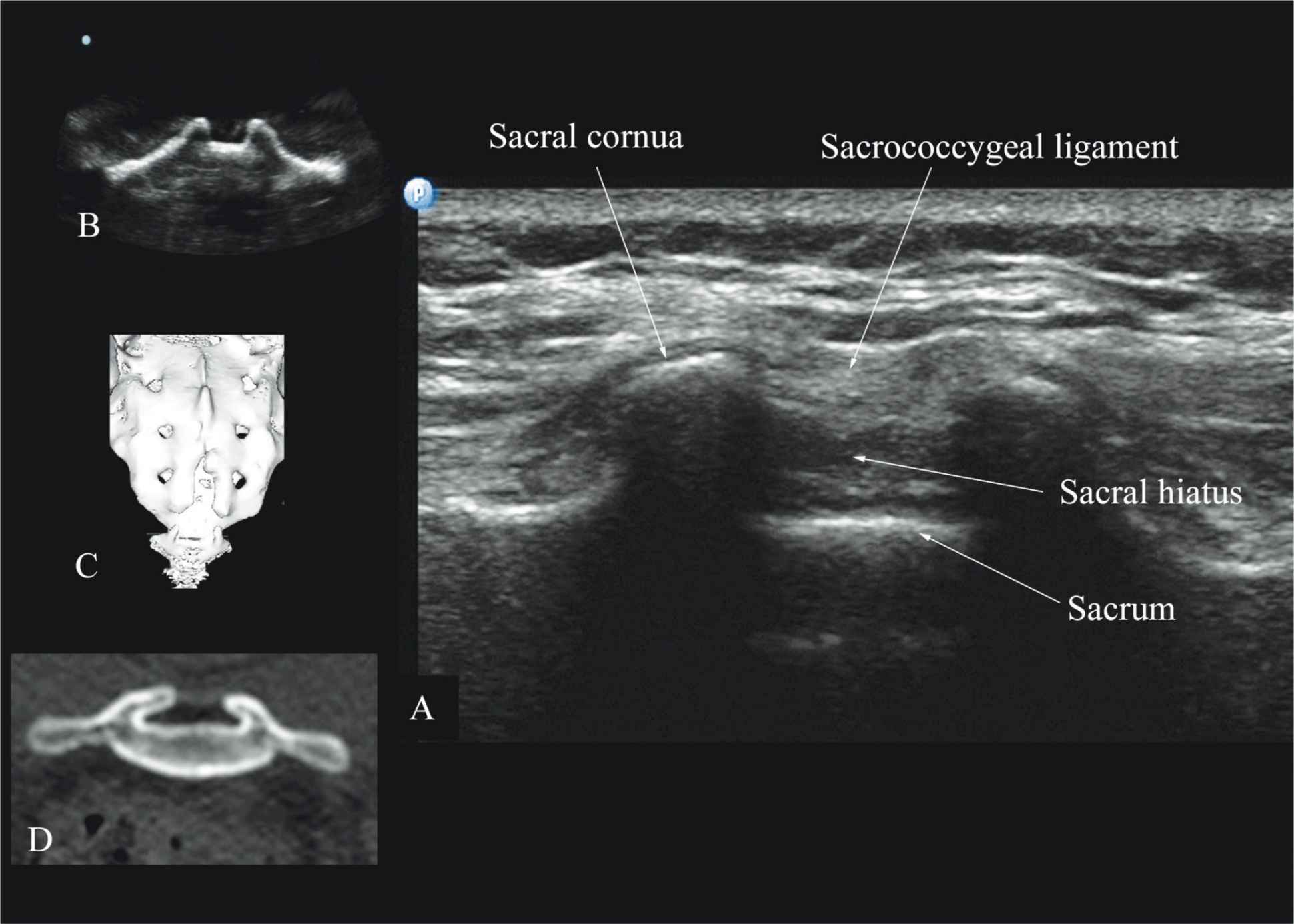
FIGURE 44-16. Transverse sonogram of the sacrum at the level of the sacral hiatus. Note the two sacral cornua and the hyperechoic sacrococcygeal ligament that extends between the two sacral cornua. The hypoechoic space between the sacrococcygeal ligament and the posterior surface of the sacrum is the sacral hiatus. Figures in the inset (B) shows the sacral cornua from the water-based spine phantom, (C) shows a three-dimensional (3D) reconstructed image of the sacrum at the level of the sacral hiatus from a 3D CT data set from the author’s archive, and (D) shows a transverse CT slice of the sacrum at the level of the sacral cornua.
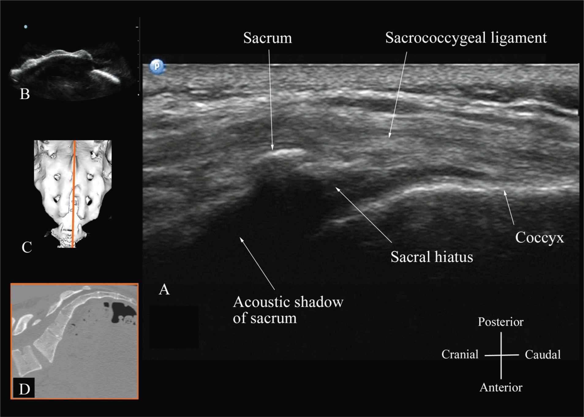
FIGURE 44-17. Sagittal sonogram of the sacrum at the level of the sacral hiatus. Note the hyperechoic sacrococcygeal ligament that extends from the sacrum to the coccyx and the acoustic shadow of the sacrum that completely obscures the sacral canal. Figures in the inset: (B) shows the sacral hiatus from the water-based spine phantom, (C) shows a three-dimensional (3D) reconstructed image of the sacrum at the level of the sacral hiatus from a 3D CT data set from the author’s archive, and (D) shows a sagittal CT slice of the sacrum at the level of the sacral cornua.
Technical Aspects of Ultrasound-Guided Central Neuraxial Blocks
“USG CNB can be performed as an off-line or in-line technique. Off-line technique involves performing a pre-puncture scan (scout scan) to preview the spinal anatomy, determine the optimal site, depth and trajectory for needle insertion before performing a traditional spinal or epidural injection.26,27 In contrast, an in-line technique involves performing a real-time USG CNB by a single17 or two4 operators.” Real-time US-guided CNB demands a high degree of manual dexterity and hand–eye coordination. Therefore, the operator should have sound knowledge of the basics of US, be familiar with the sonoanatomy of the spine and scanning techniques, and have the necessary interventional skills before attempting a real-time US-guided CNB. At this time, there are no data on the safety of the US gel if it is introduced into the meninges or the nervous tissues during US-guided regional anesthesia procedures. Therefore, it is difficult to make recommendations; although some clinicians have resorted to using a sterile normal saline solution applied using sterile swabs as an alternative coupling agent to keep the skin moist under the footprint of the transducer.17
Related posts:


Stay updated, free articles. Join our Telegram channel

Full access? Get Clinical Tree


