Fig. 10.1
Time course of plasma propofol concentrations arising from three different dosing schemes. All three time courses show the predicted plasma concentration of propofol administered at 8 mg/kg/h for 60 min without (thin solid line) or with an initial bolus of 1 mg/kg (bold dashed line) or 2 mg/kg (bold solid line). Predicted concentrations were calculated using the pharmacokinetic model developed by Marsh et al. [3]
During a constant rate infusion, the propofol plasma concentration may increase or decrease. A simulation of the time course of propofol plasma concentration after a 2 mg/kg bolus followed by an infusion at 8 mg/kg/h (bold line in Fig. 10.1) shows that the propofol plasma concentration decreases monotonically after it has reached a peak (after the end of bolus infusion) and then increases monotonically 15 min after the start of propofol administration.
Dose regimen also influences the plasma concentration during a constant rate infusion. In Fig. 10.1, the propofol plasma concentrations are different among three dose regimens, especially during the first 10 min. For example, at 8 min after the start of propofol administration, the plasma concentrations are 2.0 μg/ml if no bolus was given (thin solid line in Fig. 10.1), 2.7 μg/ml with a 1 mg/kg bolus (bold dashed line in Fig. 10.1), and 3.4 μg/ml with a 2 mg/kg bolus (bold solid line in Fig. 10.1). These examples illustrate that the context of the dosing influences the relationship between the infusion rate and plasma drug concentration.
Pharmacokinetic parameters are used to estimate plasma concentration of a drug. The following simple calculation estimates the drug concentration at steady state (Css):
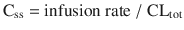
where infusion rate is the infusion rate of the drug and CLtot is the total body clearance of the drug. In anesthetic practice, this equation can be used to give a rough estimation of drug concentration. However, it is difficult to know when steady state is established.
(10.1)
Pharmacokinetic model parameters can be used to estimate the time course of drug concentration as shown in the above examples (Fig. 10.1). The following differential equations describe a three-compartment pharmacokinetic model (Fig. 10.2):
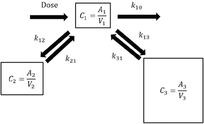
where A i is the drug amount in the ith compartment, t is the time, dose is the infusion rate of the drug at time t, k 10 is the elimination rate constant, k ij is the equilibration rate constant between the ith and jth compartments, CL i is the clearance for the ith compartment, and V i is the distribution volume of the ith compartment. Predicted concentration of a drug can be easily obtained using simulation software incorporating these equations with pharmacokinetic parameter values (pharmacokinetic model).
Fig. 10.2
Three-compartment model. A simple mathematical three-compartment pharmacokinetic model. When a drug is infused intravenously, the drug is infused into the central (the first) compartment (dose). In this compartment model, A i is the drug amount in the ith compartment, and V i is the distribution volume of the ith compartment. C i is the drug concentration in the ith compartment, calculated as A i /V i . K 10 is the elimination rate constant, and k ij is the equilibration rate constant between the ith and jth compartments. Generally, C 1 is the plasma or blood concentration of the drug. The differential equations of a three-compartment model are shown in Eq. 10.2
(10.2)
Predicted concentration is a good alternative to measured concentration of intravenous drug to see the drug concentration. The prediction of drug concentrations using pharmacokinetic models offers not only an estimation of the present concentration but also the time course of the concentration throughout the past, present, and future. Accordingly, predicted concentration helps to assess and control the drug effect in clinical practice. After assessing the concentration–clinical effect relationship of the drug using the past and present drug concentrations, the anesthesiologist can make a dosing plan using the predicted future drug concentrations.
However, there are two problems with the use of predicted plasma concentrations to control the drug effect. One is that the plasma is not the effect site for the main indications for the anesthetics or opioids (see section “PD Model and Effect-Site Concentration”). The other is that the pharmacokinetic model may not appropriately estimate the plasma concentration of the drug over time (see section “Consideration of Model Applicability”).
PD Model and Effect-Site Concentration
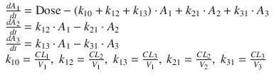
The effect site for the main effects of the anesthetics and opioids is the brain or spinal cord. Therefore, a time delay is observed in the relationship between the plasma concentration and clinical effect. Figure 10.3a clearly shows the time delay between the measured plasma concentrations of propofol and estimated BIS values [4, 5].
Fig. 10.3
The relationship between propofol concentration and propofol effect against time. (a) Time courses of measured plasma concentration of propofol and estimated propofol effect using a BIS monitor from a patient in our previous study [30]. Propofol was infused at 40 mg/kg/h for 108 s. A time delay is observed between the measured plasma concentration of propofol and estimated BIS value. (b) Time courses of effect-site concentration of propofol and estimated propofol effect using a BIS monitor in the same patient as in Fig. 10.3a. There is no time delay between the effect-site concentration and BIS value. The effect-site concentration was estimated with the raw data of measured plasma propofol concentrations and BIS values from the same patients using an effect-site pharmacodynamic model (Fig. 10.4 and Eq. 10.3) and sigmoid E max model (Eq. 10.4) [30]. In this case, an appropriate k e0 value is applied to calculate the effect-site concentration because the k e0 value was estimated for the specific individual. When a population k e0 value is used to estimate effect-site concentration, there may be a discrepancy between effect-site concentration and clinical effect because the population k e0 value may be different from individual k e0 value
To take this time delay into account, an effect-site pharmacodynamic model [6] (Fig. 10.4) can be applied using the following equation:
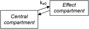
where C e is the effect-site concentration, t is the time, k e0 is the equilibration rate constant between the plasma and effect site, and C 1 is the drug concentration in the central compartment of the compartment model. If the pharmacokinetic parameters for the compartment model (all k values in Eq. 10.2) and for the effect-site model (k e0 in Eq. 10.3) are obtained, effect-site concentration can be calculated. These parameters may be found in published literature.
Fig. 10.4
Effect-compartment model . This is a simple scheme of the effect-compartment model. k e0 is the equilibration rate constant between the central compartment and the effect compartment, i.e., between the plasma concentration and the effect-site concentration of the drug. The predicted plasma concentration of the central compartment concentration is estimated by a compartment model (Fig. 10.2). Equilibration half-time may be a more intuitive concept than k e0 value, in describing the relationship between the plasma and effect-site concentrations. Equilibration half-time (t 1/2 k e0) is calculated as ln 2/k e0
(10.3)
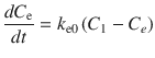
To determine the k e0 value using Eq. 10.3, the observed plasma concentrations (C 1) and effect-site concentration (C e) are necessary. However, effect-site concentration cannot be measured. Instead, the effect of the drug is observed, and an additional pharmacodynamic model such as a sigmoid E max model is applied to determine the k e0. The sigmoid E max model is described using the following equation:
where E is the observed drug effect, E 0 is the baseline measurement of the observed effect when no drug is present, E max is the maximum possible drug effect, C e is the estimated effect-site concentration, EC 50 is the effect-site concentration associated with 50 % maximum drug effect, and γ is the steepness of the effect-site concentration versus effect relationship. When applying Eqs. 10.3 and 10.4 simultaneously with the observed effect of the drug and the data of plasma concentrations, all the pharmacodynamic parameters including E 0, E max, EC 50, γ, and k e0 will be estimated.
(10.4)
The estimated k e0 value enables calculation of the time course of the effect-site concentration. There is no time delay between the effect-site concentration and the drug effect when using the appropriate k e0 value (Fig. 10.3b). In experimental settings, estimation of the k e0 value is useful for pharmacodynamic analysis. In clinical practice, an estimate of the effect-site concentration is also useful because the effect-site concentration is expected to reflect the clinical effect. However, there are limitations of the use of k e0 values for predicting effect-site concentration. One important limitation is the significant interindividual variability of the k e0 value (see section “Consideration of Effect-Site Model Application ”).
Consideration of Model Applicability
The applicability of a pharmacokinetic/pharmacodynamic model should be considered carefully when using the model for prediction. The use of an inappropriate model may cause incorrect estimations of the relationship between the drug concentration and its effect, which may increase the risk of complications such as anesthetic awareness caused by inadequate doses and concentration-related drugs side effect arising from excessive doses.
In pharmacokinetic studies, a pharmacokinetic model is developed for either prediction or description. With prediction, the model is developed to predict the drug concentration for subjects other than the subjects from whom the model was developed. With description, the model is developed to describe the measured concentrations of collected samples in a group of subjects, for a pharmacokinetic analysis, which is not intended to be used for the prediction. A model developed for description may not be suitable for prediction of drug concentrations in other subjects.
To develop an appropriate population pharmacokinetic model , model validation is generally performed to evaluate the predictability of the developed final model using a validation data set not used for building the model and parameter estimation [7]. Two types of statistically robust validations are external and internal validation. To quantify the predictability of the developed model, some metrics are applied. Visual inspection of graphical displays is also applied to evaluate the predictability.
A validated pharmacokinetic model is one with evidence for prediction of the drug concentration. However, this may still be applicable to conditions that are applied during drug administration in the subjects of the validation data set.
External Validation
External validation is the most stringent type of validation [7]. For this type of validation, two data sets are needed. One is used for the model development, and the other is for testing the external validation of the model. It is possible to apply a data set from another experiment. For the validation, metrics and/or visual inspection is applied.
There are two types of external validation. For the first type, an example might be validation of a pharmacokinetic model that has been developed from data from subjects aged 30–60 years. For this model, the predictability (external validity) may be tested using a new data set from other subjects aged 30–60 years, or subjects aged 25–65 years, or something similar to the original age range. This is a standard external validation.
The other external validation procedure is extrapolation. The validation data set should include data from subjects with focused demographics (such as age and weight) involved in a study with specific methodology condition (sampling interval or duration) which is different from the demographics or methodology involved in the model development study. This external validation of the pharmacokinetic model may expand the applicability of the model to a different population. Short et al. developed a population pharmacokinetic model of propofol using the data set obtained from 3- to 10-year-old children [8]. Sepúlveda et al. evaluated the performance of the Short pharmacokinetic model using a data set obtained from children aged 3–26 months and found that the Short model had acceptable performance [9]. This external validation study has shown that the applicability of the Short model can be expanded from the age group of the original subjects (3–10 years) to a wide age group (3 months–10 years).
Internal Validation
External validation is the most robust but needs two data sets, i.e., more subjects and samples, requiring more resources, such as man power, time, and cost, during the model development procedure. Internal validation is a method of using all the data collected data for the model development itself. Internal validation is always considered when external validation is not applied. Resampling techniques such as bootstrapping [10] and cross validation [10] and prediction-corrected visual predictive check [11] are used.
An internally validated pharmacokinetic model may be used to predict drug concentrations in patients whose age is within the range of the study population used for the model development. However, it is possible that this method of validation also involves extrapolation, because age is not the only factor that might have influenced the results of the pharmacokinetic model. Before an internally validated model is used to predict drug concentrations in a patient, it should be considered whether the patient characteristics and other dosing conditions and methods are similar to (strictly, within the range of) those used in the subjects from whom the original model was developed. The types of the factors that must be considered are explained below (see section “Subject Characteristics and Methods Used for Development of a PK Model to be Applied for Prediction”).
“Validation” or “Evaluation”
“Validation” is a strong term. A “validated” pharmacokinetic model should be suitable for prediction of drug concentrations in samples taken from subjects with different characteristics and using different dosing and study methods.
To confirm the model’s validity for various conditions, the data set for the external validation should include those conditions. However, it is common for the external validation data set to only include a limited number of the subjects under limited conditions. In other words, an external validation procedure generally only confirms a limited range of external validity.
Yano, Beal, and Sheiner proposed the use of the term of “evaluation”: “We use the weaker term ‘evaluation’ rather than the stronger one ‘validation’, as we believe one cannot truly validate a model, except perhaps in the very special case that one can both specify the complete set of alternative models that must be excluded and one has sufficient data to attain a preset degree of certainty with which these alternatives would be excluded. We believe that such cases are rare at best” [12].
Performance Error Derivatives : Metrics
Quantitative indices (metrics) are used to evaluate the population model. In the study of anesthetic pharmacology, performance error derivatives proposed by Varvel et al. [13] are frequently used. The original aim to develop the derivatives is measuring the predictive performance of computer-control infusion pumps [14–16], which is a predecessor of target-controlled infusion pumps [17].
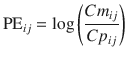
Performance Error (PE)
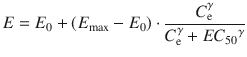
The performance error (PE, generally calculated as percentage performance error) of a model with regard to one blood sample is calculated using the following equation:
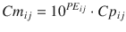
where PE ij is the performance error of jth sample in ith individual, Cm ij is the measured (observed) drug concentration of jth sample in ith individual, and Cp ij is the predicted drug concentration (using pharmacokinetic model) of jth sample in ith individual. This equation is standardized by predicted concentration. A PE value of zero means that the pharmacokinetic model predicted the concentration perfectly.
(10.5)
This standardization has several merits. When the difference between a Cm ij and a Cp ij is 1, the difference can be evaluated as small at a Cm ij of 10, whereas the difference can be evaluated as large at a Cm ij of 2. In this case, PE ij is calculated to be 11 % (Cm ij = 10 and Cp ij = 9) or 100 % (Cm ij = 2 and Cp ij = 1). The standardization quantifies the difference in a similar manner to the idea of coefficient of variation, which shows the relative variability calculated as standard deviation divided by the mean. This standardization of PE ij would be similar to the point of view of an anesthesiologist considering the drug concentration. Additionally, constant coefficient of variation models or lognormal models (similar to coefficient of variation models) as random effects is used to describe interindividual and intraindividual variability in population models [18]. This is one advantage of using PE ij .
Another further strength is that predicted concentrations, and not measured concentrations, are used as standard. In clinical and research work, clinicians and researchers are almost always dealing with predicted concentrations instead of measured concentration. Therefore, the use of predicted concentration as standard is reasonable.
During model evaluation, the term “prediction error ” may be used instead of “performance error.” With respect to this term, the equations of PE and PE derivatives are the same.
In standard pharmacometrics, the performance error is calculated as ODV minus PDV, where ODV is the value of the observed dependent variable, e.g., observed drug concentration, and PDV is the value of the predicted dependent variable. This is the same concept as used in an additive error model for interindividual and intraindividual variability in population models [18].
Performance Error Derivatives and Visual Inspection of the Model
There are four original performance error derivatives, namely, median absolute performance error (MDAPE ), median performance error (MDPE), divergence, and wobble.
MDAPE indicates the inaccuracy of the prediction. In the ith subject,
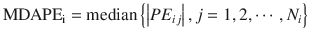
where MDAPEi is MDAPE of the ith subject, PE ij is the performance error of the jth sample in the ith subject (Eq. 10.5), and N i is the number of |PE| values obtained from the ith subject. The closer to zero the MDAPE i , the more accurate the model for prediction of concentrations in the ith individual.
(10.6)
MDPE reflects the bias of the prediction. In the ith subject:
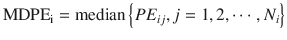
where MDPEi is MDPE of the ith subject, PE ij is the performance error of the jth sample in the ith subject (Eq. 10.5), and N i is the number of PE values obtained from the ith subject. An MDPEi of zero means that the model has no bias in its prediction of concentrations in the ith subject. An MDPE larger or smaller than zero indicates underprediction (i.e., measured concentration > predicted concentration) or overprediction (i.e., predicted concentration > measured concentration), respectively.
(10.7)
Divergence shows the rate of change of absolute performance error against time. Divergencei (generally expressed in %/h) is calculated as the slope of the linear regression of absolute performance error versus time. A negative value of divergence indicates that the predicted concentration comes closer to measured concentration over time.
Wobble quantifies the intraindividual variability of the prediction error. In the ith subject:
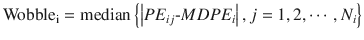
where Wobblei is wobble of the ith subject, PE ij is the performance error of the jth sample in the ith subject (Eq. 10.5), MDPE i is the median performance error in the ith subject (Eq. 10.7), and N i is the number of PE values obtained from the ith subject. The smaller value of the wobble, the more stable the predictions of the pharmacokinetic model.
(10.8)
The population estimate for each of these performance error derivatives is generally calculated as the mean of the individual estimates . For example, population MDPE is calculated using the following equation:
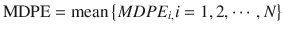
where MDPE i is MDPE of the ith subject and N is the number of the subjects in the population.
(10.9)
Two Types of Divergence
As mentioned above, the original divergence parameter proposed by Varvel was the measure of divergence of APE , calculated as the slope of the linear regression of absolute performance error over time. Since then another divergence parameter has been proposed, which is divergence in PE, calculated as the slope of the linear regression of performance error over time [19]. Glen et al. proposed the use of both divergence parameters to evaluate the predictive performance of pharmacokinetic models [19]. Divergence APE and divergence PE reveal different information and may result in seemingly contradictory evaluations of a model as shown and explained in Fig. 10.5.
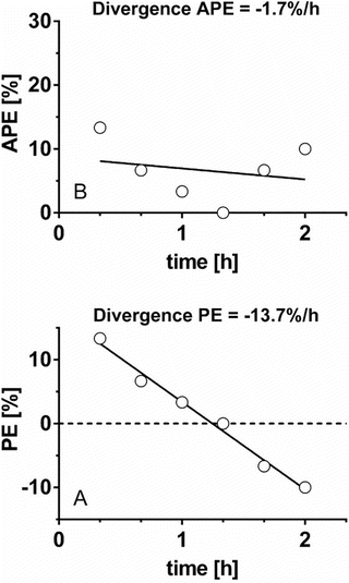
Fig. 10.5
Two types of divergence. Six absolute performance errors (APE ) and performance errors (PE) obtained from six pairs of measured and predicted drug concentrations during 2 h are depicted in a and b, respectively. For this data set, original divergence (divergence APE ) is −1.7 %/h, which indicates that the APE decreases to zero versus time, i.e., predicted concentration is getting closer to measured concentration as time progresses. On the other hand, divergence PE is −13.7 %/h, which indicates PE decreases 13.7 %/h over time. The decrement of PE means that measured concentration decreases against predicted concentration over time. When the drug is administered using target-controlled infusion, measured concentration gradually decreases. Therefore, a pharmacokinetic model with large negative divergence PE is associated with an increased risk of insufficient drug effect. The two types of divergence, original divergence (divergence APE ) and divergence PE, provide different information
Acceptable Ranges of PE Derivatives
An MDPE between −20 and 20 % and an MDAPE <30 % during target-controlled infusion are regarded as acceptable [20, 21]. These can be used as criteria for external evaluation of a model. In many studies evaluating the accuracy of model prediction [9, 22, 23], expected performance of drug delivery devices such as target-controlled infusion pumps tends to be an MDPE of around 20–30 % [24].
There are no published criteria for acceptable values of divergence and wobble. A divergence APE <3–5 %/h and divergence PE between −5 and −3 %/h and between 3 and 5 %/h may be acceptable. A divergence APE of 3–5 %/h means absolute performance error increases 30–50 % over 10 h. A larger than 50 % increase of APE seems to be unacceptable. For target-controlled infusions of propofol, positive divergence PE is more preferable than negative one. As a negative divergence PE means that PE decreases against time, implying that the measured concentration is decreasing relative to the predicted concentration, there is a risk of awareness in this case.
It is difficult to define an acceptable value of wobble because not only will the accuracy and relevance of the prediction model parameters influence performance, but wobble may also be influenced by physiological factors such as cardiac output or uncompensated bleeding [25–27] that may increase the intraindividual variability of the prediction. By definition the wobble value will be less than MDAPE (Eq. 10.8).
Limitation of Performance Error Standardized by Predicted Concentration
As explained above, there are both advantages and disadvantages of using performance error standardized by predicted concentration (Eq. 10.5).
Performance error has a minimum value of −100 % when the measured concentration is zero but can theoretically be infinitely large (e.g., when a measured value is high, while the predicted value is close to zero). This means that the evaluation using this PE is asymmetric with respect to overprediction and underprediction. For example, consider the two combinations of measured and predicted concentrations, respectively, “2 μg/ml and 3 μg/ml” (overprediction) versus “3 μg/ml and 2 μg/ml” (underprediction). For the overprediction combination, the prediction error is −33.3 %, whereas for the underprediction combination the prediction error is 50 %. When using performance error standardized by predicted concentration (Eq. 10.5), a model overestimating the concentration tends to be assessed as better than a model underestimating the concentration. This estimation tendency is preferable to avoid higher (but not lower) measured concentrations.
Possible Alternatives of Performance Error
To obtain symmetry in the performance error, a modification of performance error, or another index, is necessary.
We previously developed another index as an alternative to performance error defined using the Eq. 10.5. During the evaluation of a pharmacokinetic model, plots are often made of Cm/Cp (the ratio of measured to predicted concentrations) displayed against a variable such as time or predicted concentration. These plots are often described as goodness of fit plots (explained in the next section) [22, 28, 29]. For these plots, a logarithmic y-axis is used for Cm/Cp. On any logarithmic axis, by definition Y and 1/Y are symmetrical because y = Y and y = 1/Y are equidistant from y = 1. Accordingly, we proposed the log-transformed value of Cm/Cp as a new index [22]. To calculate this index, the following equation is applied:
where PE ij is the performance error of jth sample in ith individual, Cm ij is the measured (observed) drug concentration of jth sample in ith individual, and Cp ij is the predicted drug concentration of jth sample in ith individual. When a pharmacokinetic model predicts a single sample perfectly (i.e., Cm ij = Cp ij ), prediction error is 0, which is the same value for perfect prediction using Eq. 10.5. For all imperfect predictions , the performance errors calculated by Eqs. 10.5 and 10.10 are different.
(10.10)
Equation 10.10 can be rearranged to:
A value of 1 for PE ij means that Cm ij is ten times Cp ij , and a value of −1 means that Cm ij is one-tenth of Cp ij . The PE values calculated using Eq. 10.10 are distributed symmetrically on a linearly scaled axis (not logarithmic axis). Using this logarithmic transformation, we can calculate PE derivatives of MDAPE (Eq. 10.6), MDPE (Eq. 10.7), divergences (divergence APE and divergence PE), and wobble (Eq. 10.8).
(10.11)
The meaning of the ratio Cm/Cp is intuitive. However, the values of PE calculated using either Eqs. 10.5 or 10.10 are quite different, e.g., when Cm is 4.5 and Cp is 3, PE is calculated to be 50 % by Eq. 10.5 or to be 0.18 by Eq. 10.10 (Fig. 10.6). Therefore, it is difficult to compare PE derivatives from Eq. 10.10 with ones calculated from Eq. 10.5 [22].
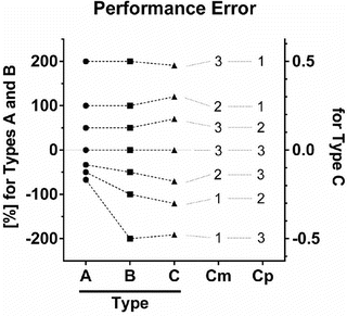
Fig. 10.6
Three types of performance error. The following are three different equations for calculation of the performance error (PE): A (Eq. 10.5) 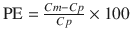 , B (Eq. 10.12)
 ![$$ \mathrm{P}\mathrm{E}=\left\{\begin{array}{c}\hfill \frac{Cm- Cp}{Cp}\times 100\kern0.48em \left[\mathrm{if}\; Cm\ge Cp\right]\hfill \\ {}\hfill \frac{Cm- Cp}{Cm}\times 100\kern0.48em \left[\mathrm{if}\; Cm< Cp\right]\hfill \end{array}\right. $$](/wp-content/uploads/2017/07/A339434_1_En_10_Chapter_IEq2.gif) , C (Eq. 10.10)
, C (Eq. 10.10) 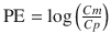 , where Cm is the measured (observed) concentration and Cp is the predicted concentration estimated using a pharmacokinetic model. Each circle, square, and triangle indicates each PE value
, B (Eq. 10.12) , C (Eq. 10.10) , where Cm is the measured (observed) concentration and Cp is the predicted concentration estimated using a pharmacokinetic model. Each circle, square, and triangle indicates each PE valueAnother PE definition can be considered:
![$$ {\mathrm{PE}}_{ij}=\left\{\begin{array}{c}\hfill \frac{C{m}_{ij}- C{p}_{ij}}{C{p}_{ij}}\times 100\kern0.36em \left[\mathrm{if}\; C{m}_{ij}\ge C{p}_{ij}\right]\hfill \\ {}\hfill \frac{C{m}_{ij}- C{p}_{ij}}{C{m}_{ij}}\times 100\kern0.36em \left[\mathrm{if}\; C{m}_{ij}< C{p}_{ij}\right]\hfill \end{array}\right. $$](/wp-content/uploads/2017/07/A339434_1_En_10_Chapter_Equ12.gif)
where PE ij is the performance error of jth sample in ith individual, Cm ij is the measured (observed) drug concentration of jth sample in ith individual, and Cp ij is the predicted drug concentration of jth sample in ith individual. The first equation is the same as Eq. 10.5. The second equation is added for the symmetry . For example, with this approach, the two combinations of measured and predicted concentrations, “2 and 3” (over prediction) and “3 and 2” (underprediction), are symmetric. For these concentration combinations, the prediction errors are −33.3 % and 33.3 %, respectively, using Eq. 10.12 (the latter prediction error is calculated to be 50 % using Eq. 10.5).
(10.12)
Figure 10.6 shows the performance error distribution of different concentration combinations. With the PE defined by Eq. 10.5 (Fig. 10.6, Type A), the distribution of the PE is asymmetric with respect to the zero value of PE. On the other hand, the distribution of PEs is symmetric, when PE is defined according to Eq. 10.12 (Fig. 10.6, Type B) or Eq. 10.10 (Fig. 10.6, Type C). Only the PE values defined by Eq. 10.5 have a lower boundary (as mentioned the minimum value is −100 %).
For PEs calculated using Eq. 10.5 (Fig. 10.6, Type A) and Eq. 10.12 (Fig. 10.6, Type B), the PE values are completely the same for any combination of Cm and Cp resulting in PE ≥ 0. For example in Fig. 10.6, the circle or square for the combination of “Cm = 2” and “Cp = 1” resulting in PE of 100 % has the same distance from the gray line for PE of zero (meaning perfect prediction). On the other hand, the PE value is different for any combination of Cm and Cp resulting in PE < 0. For example in Fig. 10.6, the PE values for the combination of “Cm = 1” and “Cp = 2” are −50 % with Eq. 10.5 (Fig. 10.6, Type A) and −100 % with Eq. 10.12 (Fig. 10.6, Type B) resulting in different distances from the gray line for PE of zero.
Related posts:


Stay updated, free articles. Join our Telegram channel

Full access? Get Clinical Tree


