Experimental Design and Statistics
Nathan Leon Pace
Key Points
Related Matter
Graphing Data
Introduction
If a physician is to be a practitioner of scientific medicine, he or she must read the language of science to be able to independently assess and interpret the scientific report. Without exception, the language of the medical report is increasingly statistical. Readers of the anesthesia literature, whether in a community hospital or a university environment, cannot and should not totally depend on the editors of journals to banish all errors of statistical analysis and interpretation. In addition, there are regularly questions about simple statistics in examinations required for anesthesiologists. Finally, certain statistical methods have everyday applications in clinical medicine. This chapter briefly scans some elements of experimental design and statistical analysis.
Design of Research Studies
Sampling
Two words of great importance to statisticians are population and sample. In statistical language, each has a specialized meaning. Instead of referring only to the count of individuals in a geographic or political region, population refers to any target group of things (animate or inanimate) in which there is interest. For anesthesia researchers, a typical target population might be mothers in the first stage of labor or head-trauma victims undergoing craniotomy. A target population could also be cell cultures, isolated organ preparations, or hospital bills. A sample is a subset of the target population. Samples are taken because of the impossibility of observing the entire population; it is generally not affordable, convenient, or practical to examine more than a relatively small fraction of the population. Nevertheless, the researcher wishes to generalize from the results of the small sample group to the entire population.
Although the subjects of a population are alike in at least one way, these population members are generally quite diverse in other ways. Because the researcher can work only with a subset of the population, he or she hopes that the sample of subjects in the experiment is representative of the population’s diversity. Head-injury patients can have open or closed wounds, a variety of coexisting diseases, and normal or increased intracranial pressure. These subgroups within a population are called strata. Often the researcher wishes to increase the sameness or homogeneity of the target population by further restricting it to just a few strata; perhaps only closed and not open head injuries will be included. Restricting the target population to eliminate too much diversity must be balanced against the desire to have the results be applicable to the broadest possible population of patients.
The best hope for a representative sample of the population would be realized if every subject in the population had the same chance of being in the experiment; this is called random sampling. If there were several strata of importance, random sampling from each stratum would be appropriate. Unfortunately, in most clinical anesthesia studies researchers are limited to using those patients who happen to show up at their hospitals; this is called convenience sampling. Convenience sampling is also subject to the nuances of the surgical schedule, the goodwill of the referring physician and attending surgeon, and the willingness of the patient to cooperate. At best, the convenience sample is representative of patients at that institution, with no assurance that these patients are similar to those elsewhere. Convenience sampling is also the rule in studying new anesthetic drugs; such studies are typically performed on healthy, young volunteers.
Experimental Constraints
The researcher must define the conditions to which the sample members will be exposed. Particularly in clinical research, one must decide whether these conditions should be rigidly standardized or whether the experimental circumstances should be adjusted or individualized to the patient. In anesthetic drug research, should a fixed dose be given to all members of the sample or should the dose be adjusted to produce an effect or to achieve a specific end point? Standardizing the treatment groups by fixed doses simplifies the research work. There are risks to this standardization, however (1) a fixed dose may produce excessive numbers of side effects in some patients; (2) a fixed dose may be therapeutically insufficient in others; and (3) a treatment standardized for an experimental protocol may be so artificial that it has no broad clinical relevance, even if demonstrated to be superior. The researcher should carefully choose and report the adjustment/individualization of experimental treatments.
Control Groups
the effects of the drug under related but not necessarily identical circumstances could be used. Under the first two possibilities, the control group is contemporaneous—either a self-control (crossover) or parallel control group. The second two possibilities are examples of the use of historical controls.
Since historical controls already exist, they are convenient and seemingly cheap to use. Unfortunately, the history of medicine is littered with the “debris” of therapies enthusiastically accepted on the basis of comparison with past experience. A classic example is operative ligation of the internal mammary artery for the treatment of angina pectoris—a procedure now known to be of no value. Proposed as a method to improve coronary artery blood flow, the lack of benefit was demonstrated in a trial where some patients had the procedure and some had a sham procedure; both groups showed benefit.1 There is now firm empirical evidence that studies using historical controls usually show a favorable outcome for a new therapy, whereas studies with concurrent controls, that is, parallel control group or self-control, less often reveal a benefit.2 Nothing seems to increase the enthusiasm for a new treatment as much as the omission of a concurrent control group. If the outcome with an old treatment is not studied simultaneously with the outcome of a new treatment, one cannot know if any differences in results are a consequence of the two treatments, or of unsuspected and unknowable differences between the patients, or of other changes over time in the general medical environment. One possible exception would be in studying a disease that is uniformly fatal (100% mortality) over a very short time.
Random Allocation of Treatment Groups
Having accepted the necessity of an experiment with a control group, the question arises as to the method by which each subject should be assigned to the predetermined experimental groups. Should it depend on the whim of the investigator, the day of the week, the preference of a referring physician, the wish of the patient, the assignment of the previous subject, the availability of a study drug, a hospital chart number, or some other arbitrary criterion? All such methods have been used and are still used, but all can ruin the purity and usefulness of the experiment. It is important to remember the purpose of sampling: By exposing a small number of subjects from the target population to the various experimental conditions, one hopes to make conclusions about the entire population. Thus, the experimental groups should be as similar as possible to each other in reflecting the target population; if the groups are different, selection bias is introduced into the experiment. Although randomly allocating subjects of a sample to one or another of the experimental groups requires additional work, this principle prevents selection bias by the researcher, minimizes (but cannot always prevent) the possibility that important differences exist among the experimental groups, and disarms the critics’ complaints about research methods. Random allocation is most commonly accomplished by the use of computer-generated random numbers. Even with a random allocation process, selection bias can occur if research personnel are allowed knowledge of the group assignment of the next patient to be recruited for a study. Failure to conceal random allocation leads to biases in the results of clinical studies.3,4
Blinding
Blinding refers to the masking from the view of patient and experimenters the experimental group to which the subject has been or will be assigned. In clinical trials, the necessity for blinding starts even before a patient is enrolled in the research study; this is called the concealment of random allocation. There is good evidence that, if the process of random allocation is accessible to view, the referring physicians, the research team members, or both are tempted to manipulate the entrance of specific patients into the study to influence their assignment to a specific treatment group5; they do so having formed a personal opinion about the relative merits of the treatment groups and desiring to get the “best” for someone they favor. This creates bias in the experimental groups.
Each subject should remain, if possible, ignorant of the assigned treatment group after entrance into the research protocol. The patient’s expectation of improvement, a placebo effect, is a real and useful part of clinical care. But when studying a new treatment, one must ensure that the fame or infamy of the treatments does not induce a bias in outcome by changing patient expectations. A researcher’s knowledge of the treatment assignment can bias his or her ability to administer the research protocol and to observe and record data faithfully; this is true for clinical, animal, and in vitro research. If the treatment group is known, those who observe data cannot trust themselves to record the data impartially and dispassionately. The appellations single-blind and double-blind to describe blinding are commonly used in research reports, but often applied inconsistently; the researcher should carefully plan and report exactly who is blinded.
Types of Research Design
Ultimately, research design consists of choosing what subjects to study, what experimental conditions and constraints to enforce, and which observations to collect at what intervals. A few key features in this research design largely determine the strength of scientific inference on the collected data. These key features allow the classification of research reports (Table 9-1). This classification reveals the variety of experimental approaches and indicates strengths and weaknesses of the same design applied to many research problems.
The first distinction is between longitudinal and cross-sectional studies. The former is the study of changes over time, whereas the latter describes a phenomenon at a certain point in time. For example, reporting the frequency with which certain drugs are used during anesthesia is a cross-sectional study, whereas investigating the hemodynamic effects of different drugs during anesthesia is a longitudinal one.
Longitudinal studies are next classified by the method with which the research subjects are selected. These methods for choosing research subjects can be either prospective or retrospective; these two approaches are also known as cohort (prospective) or
case-control (retrospective). A prospective study assembles groups of subjects by some input characteristic that is thought to change an output characteristic; a typical input characteristic would be the opioid drug administered during anesthesia; for example, remifentanil or fentanyl. A retrospective study gathers subjects by an output characteristic; an output characteristic is the status of the subject after an event; for example, the occurrence of a myocardial infarction. A prospective (cohort) study would be one in which a group of patients undergoing neurologic surgery was divided in two groups, given two different opioids (remifentanil or fentanyl), and followed for the development of a perioperative myocardial infarction. In a retrospective (case-control) study, patients who suffered a perioperative myocardial infarction would be identified from hospital records; a group of subjects of similar age, gender, and disease who did not suffer a perioperative myocardial infarction would also be chosen, and the two groups would then be compared for the relative use of the two opioids (remifentanil or fentanyl). Retrospective studies are a primary tool of epidemiology. A case-control study can often identify an association between an input and an output characteristic, but the causal link or relationship between the two is more difficult to specify.
case-control (retrospective). A prospective study assembles groups of subjects by some input characteristic that is thought to change an output characteristic; a typical input characteristic would be the opioid drug administered during anesthesia; for example, remifentanil or fentanyl. A retrospective study gathers subjects by an output characteristic; an output characteristic is the status of the subject after an event; for example, the occurrence of a myocardial infarction. A prospective (cohort) study would be one in which a group of patients undergoing neurologic surgery was divided in two groups, given two different opioids (remifentanil or fentanyl), and followed for the development of a perioperative myocardial infarction. In a retrospective (case-control) study, patients who suffered a perioperative myocardial infarction would be identified from hospital records; a group of subjects of similar age, gender, and disease who did not suffer a perioperative myocardial infarction would also be chosen, and the two groups would then be compared for the relative use of the two opioids (remifentanil or fentanyl). Retrospective studies are a primary tool of epidemiology. A case-control study can often identify an association between an input and an output characteristic, but the causal link or relationship between the two is more difficult to specify.
Table 9-1. Classification of Clinical Research Reports | |
|---|---|
|
Prospective studies are further divided into those in which the investigator performs a deliberate intervention and those in which the investigator merely observes. In a study of deliberate intervention, the investigator would choose several anesthetic maintenance techniques and compare the incidence of postoperative nausea and vomiting. If it were performed as an observational study, the investigator would observe a group of patients receiving anesthetics chosen at the discretion of each patient’s anesthesiologist and compare the incidence of postoperative nausea and vomiting (PONV) among the anesthetics used. Obviously, in this example of an observational study, there has been an intervention; an anesthetic has been given. The crucial distinction is whether the investigator controlled the intervention. An observational study may reveal differences among treatment groups, but whether such differences are the consequence of the treatments or of other differences among the patients receiving the treatments will remain obscure.
Studies of deliberate intervention are further subdivided into those with concurrent controls and those with historical controls. Concurrent controls are either a simultaneous parallel control group or a self-control study; historical controls include previous studies and literature reports. A randomized controlled trial (RCT) is thus a longitudinal, prospective study of deliberate intervention with concurrent controls.
Although most of this discussion about experimental design has focused on human experimentation, the same principles apply and should be followed in animal experimentation. The randomized, controlled clinical trial is the most potent scientific tool for evaluating medical treatment; randomization into treatment groups is relied on to equally weight the subjects of the treatment groups for baseline attributes that might predispose or protect the subjects from the outcome of interest.
Data and Descriptive Statistics
Statistics is a method for working with sets of numbers, a set being a group of objects. Statistics involves the description of number sets, comparison of number sets with theoretical models, comparison between number sets, and comparison of recently acquired number sets with those from the past. A typical scientific hypothesis asks which of two methods (treatments), X and Y, is better. A statistical hypothesis is formulated concerning the sets of numbers collected under the conditions of treatments X and Y. Statistics provides methods for deciding if the set of values associated with X are different from the values associated with Y. Statistical methods are necessary because there are sources of variation in any data set, including random biologic variation and measurement error. These errors in the data cause difficulties in avoiding bias and in being precise. Bias keeps the true value from being known and fosters incorrect decisions; precision deals with the problem of the data scatter and with quantifying the uncertainty about the value in the population from which a sample is drawn. These statistical methods are relatively independent of the particular field of study. Regardless of whether the numbers in sets X and Y are systolic pressures, body weights, or serum chlorides, the approach for comparing sets X and Y is usually the same.
Data Structure
Data collected in an experiment include the defining characteristics of the experiment and the values of events or attributes that vary over time or conditions. The former are called explanatory variables and the latter are called response variables. The researcher records his or her observations on data sheets or case record forms, which may be one to many pages in length, and assembles them together for statistical analysis. Variables such as gender, age, and doses of accompanying drugs reflect the variability of the experimental subjects. Explanatory variables, it is hoped, explain the systematic variations in the response variables. In a sense, the response variables depend on the explanatory variables.
Response variables are also called dependent variables. Response variables reflect the primary properties of experimental interest in the subjects. Research in anesthesiology is particularly likely to have repeated measurement variables; that is, a particular measurement recorded more than once for each individual. Some variables can be both explanatory and response; these are called intermediate response variables. Suppose an experiment is conducted comparing electrocardiography and myocardial responses between five doses of an opioid. One might analyze how ST segments depended on the dose of opioids; here, maximum ST segment depression is a response variable. Maximum ST segment depression might also be used as an explanatory variable to address the subtler question of the extent to which the effect of an opioid dose on postoperative myocardial infarction can be accounted for by ST segment changes.
The mathematical characteristics of the possible values of a variable fit into five classifications (Table 9-2). Properly assigning a variable to the correct data type is essential for choosing the correct statistical technique. For interval variables, there is equal distance between successive intervals; the difference between 15 and 10 is the same as the difference between 25 and 20. Discrete interval data can have only integer values; for example, number of living children. Continuous interval data are measured on a continuum and can be a decimal fraction; for example, blood pressure can be described as accurately as desired (e.g., 136, 136.1, or 136.14 mm Hg). The same statistical techniques are used for discrete and continuous data.
Putting observations into two or more discrete categories derives categorical variables; for statistical analysis, numeric values are assigned as labels to the categories. Dichotomous data allow only two possible values; for example, male versus female. Ordinal data have three or more categories that can logically be ranked or ordered; however, the ranking or ordering of the variable indicates only relative and not absolute differences between values; there is not necessarily the same difference between American Society of Anesthesiologists Physical Status score I and II as there
is between III and IV. Although ordinal data are often treated as interval data in choosing a statistical technique, such analysis may be suspect; alternative techniques for ordinal data are available. Nominal variables are placed into categories that have no logical ordering. The eye colors blue, hazel, and brown might be assigned the numbers 1, 2, and 3, but it is nonsense to say that blue < hazel < brown.
is between III and IV. Although ordinal data are often treated as interval data in choosing a statistical technique, such analysis may be suspect; alternative techniques for ordinal data are available. Nominal variables are placed into categories that have no logical ordering. The eye colors blue, hazel, and brown might be assigned the numbers 1, 2, and 3, but it is nonsense to say that blue < hazel < brown.
Table 9-2. Data Types | ||||||||||||||||||||||||
|---|---|---|---|---|---|---|---|---|---|---|---|---|---|---|---|---|---|---|---|---|---|---|---|---|
|
Descriptive Statistics
|
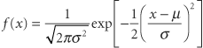 There are two parameters (population mean and population variance) in the equation of the normal function that are denoted μ and σ2. Often called the normal equation, it can be plotted and produces the familiar bell-shaped curve. Why are the mathematical properties of this curve so important to biostatistics? First, it has been empirically noted that when a biologic variable is sampled repeatedly, the pattern of the numbers plotted as a histogram resembles the normal curve; thus, most biologic data are said to follow or to obey a normal distribution. Second, if it is reasonable to assume that a sample is from a normal population, the mathematical properties of the normal equation can be used with the sampling statistic estimators of the population parameters to describe the sample and the population. Third, a mathematical theorem (the central limit theorem) allows the use of the assumption of normality for certain purposes, even if the population is not normally distributed.
Central Location
|
 where i is the index of summation and n is the count of objects in the sample. If all values in the population could be obtained, then the population mean μ could be calculated similarly. Since all values of the population cannot be obtained, the sample mean is used. (Statisticians describe the sample mean as the unbiased, consistent, minimum variance, sufficient estimator of the population mean. Estimators are denoted by a hat over a greek letter; for example,
  . Thus, the sample mean [x with bar above] is the estimator
  of the population mean μ.)
The median is the middlemost number or the number that divides the sample into two equal parts—first, ranking the sample values from lowest to highest and then counting up halfway to obtain the median. The concept of ranking is used in nonparametric statistics. A virtue of the median is that it is hardly affected by a few extremely high or low values. The mode is the most popular number of a sample; that is, the number that occurs most frequently. A sample may have ties for the most common value and be bi- or polymodal; these modes may be widely separated or adjacent. The raw data should be inspected for this unusual appearance. The mode is always mentioned in discussions of descriptive statistics, but it is rarely used in statistical practice.
Spread or Variability
Any set of interval data has variability unless all the numbers are identical. The range of ages from lowest to highest expresses the largest difference. This spread, diversity, and variability can also be expressed in a concise manner. Variability is specified by calculating the deviation or deviate of each individual xi from the center (mean) of all the xi‘s. The sum of the squared deviates is always positive unless all set values are identical. This sum is then divided by the number of individual measurements. The result is
the averaged squared deviation; the average squared deviation is ubiquitous in statistics.
the averaged squared deviation; the average squared deviation is ubiquitous in statistics.
The concept of describing the spread of a set of numbers by calculating the average distance from each number to the center of the numbers applies to both a sample and a population; this average squared distance is called the variance. The population variance is a parameter and is represented by σ2. As with the population mean, the population variance is not usually known and cannot be calculated. Just as the sample mean is used in place of the population mean, the sample variance is used in place of the population variance. The sample variance is
Statistical theory demonstrates that if the divisor in the formula for SD2 is (n – 1) rather than n, the sample variance is an unbiased estimator of the population variance. While the variance is used extensively in statistical calculations, the units of variance are squared units of the original observations. The square root of the variance has the same units as the original observations; the square roots of the sample and population variances are called the sample (SD) and population (σ) standard deviations.
It was previously mentioned that most biologic observations appear to come from populations with normal distributions. By accepting this assumption of a normal distribution, further meaning can be given to the sample summary statistics (mean and SD) that have been calculated. This involves the use of the expression [x with bar above] ± k × SD, where k = 1, 2, 3, and so forth. If the population from which the sample is taken is unimodal and roughly symmetric, then the bounds for 1, 2, and 3 encompasses roughly 68%, 95%, and 99% of the sample and population members.
Hypotheses and Parameters
Hypothesis Formulation
The researcher starts work with some intuitive feel for the phenomenon to be studied. Whether stated explicitly or not, this is the biologic hypothesis; it is a statement of experimental expectations to be accomplished by the use of experimental tools, instruments, or methods accessible to the research team. An example would be the hope that isoflurane would produce less myocardial ischemia than fentanyl; the experimental method might be the electrocardiography determination of ST segment changes. The biologic hypothesis of the researcher becomes a statistical hypothesis during research planning. The researcher measures quantities that can vary—variables such as heart rate or temperature or ST segment change—in samples from populations of interest. In a statistical hypothesis, statements are made about the relationship among parameters of one or more populations. (To restate, a parameter is a number describing a variable of a population; Greek letters are used to denote parameters.) The typical statistical hypothesis can be established in a somewhat rote fashion for every research project, regardless of the methods, materials, or goals. The most frequently used method of setting up the algebraic formulation of the statistical hypothesis is to create two mutually exclusive statements about some parameters of the study population (Table 9-3); estimates for the values for these parameters are acquired by sampling data. In the hypothetical example comparing isoflurane and fentanyl, φ1 and φ2 would represent the ST segment changes with isoflurane and with fentanyl. The null hypothesis is the hypothesis of no difference of ST segment changes between isoflurane and fentanyl. The alternative hypothesis is usually nondirectional, that is, either φ1 < φ2 or φ1 > φ2; this is known as a two-tail alternative hypothesis. This is a more conservative alternative hypothesis than assuming that the inequality can only be either less than or greater than.
Table 9-3. Algebraic Statement of Statistical Hypotheses | ||||
|---|---|---|---|---|
|
Logic of Proof
One particular decision strategy is used most commonly to choose between the null and the alternative hypothesis. The decision strategy is similar to a method of indirect proof used in mathematics called reductio ad absurdum (proof by contradiction). If a theorem cannot be proved directly, assume that it is not true; show that the falsity of this theorem will lead to contradictions and absurdities; thus, reject the original assumption of the falseness of the theorem. For statistics, the approach is to assume that the null hypothesis is true even though the goal of the experiment is to show that there is a difference. One examines the consequences of this assumption by examining the actual sample values obtained for the variable(s) of interest. This is done by calculating what is called a sample test statistic; sample test statistics are calculated from the sample numbers. Associated with a sample test statistic is a probability. One also chooses the level of significance; the level of significance is the probability level considered too low to warrant support of the null hypothesis being tested. If sample values are sufficiently unlikely to have occurred by chance (i.e., the probability of the sample test statistic is less than the chosen level of significance), the null hypothesis is rejected; otherwise, the null hypothesis is not rejected.
Because the statistics deal with probabilities, not certainties, there is a chance that the decision concerning the null hypothesis is erroneous. These errors are best displayed in table form (Table 9-4); condition 1 and condition 2 could be different drugs, two doses of the same drug, or different patient groups. Of the four possible outcomes, two decisions are clearly undesirable. The error of wrongly rejecting the null hypothesis (false positive) is called the type I or alpha error. The experimenter should choose a probability value for alpha before collecting data; the experimenter decides how cautious to be against falsely claiming a difference. The most common choice for the value of alpha is 0.05. What are the consequences of choosing an alpha of 0.05? Assuming that there is, in fact, no difference between the two conditions and that the experiment is to be repeated 20 times, then during one of these experimental replications (5% of 20) a mistaken conclusion that there is a difference would be made. The probability of a type I error depends on the chosen level of significance and the existence or nonexistence of a difference between the two experimental conditions. The smaller the chosen alpha, the smaller will be the risk of a type I error.
The error of failing to reject a false null hypothesis (false negative) is called a type II or beta error. (The power of a test is 1 minus beta). The probability of a type II error depends on four factors.
Unfortunately, the smaller the alpha, the greater the chance of a false-negative conclusion; this fact keeps the experimenter from automatically choosing a very small alpha. Second, the more variability there is in the populations being compared, the greater the chance of a type II error. This is analogous to listening to a noisy radio broadcast; the more static there is, the harder it will be to discriminate between words. Next, increasing the number of subjects will lower the probability of a type II error. The fourth and most important factor is the magnitude of the difference between the two experimental conditions. The probability of a type II error goes from very high, when there is only a small difference, to extremely low, when the two conditions produce large differences in population parameters.
Unfortunately, the smaller the alpha, the greater the chance of a false-negative conclusion; this fact keeps the experimenter from automatically choosing a very small alpha. Second, the more variability there is in the populations being compared, the greater the chance of a type II error. This is analogous to listening to a noisy radio broadcast; the more static there is, the harder it will be to discriminate between words. Next, increasing the number of subjects will lower the probability of a type II error. The fourth and most important factor is the magnitude of the difference between the two experimental conditions. The probability of a type II error goes from very high, when there is only a small difference, to extremely low, when the two conditions produce large differences in population parameters.
Table 9-4. Errors in Hypothesis Testing: The Two-Way Truth Table | ||||||||||||||||||
|---|---|---|---|---|---|---|---|---|---|---|---|---|---|---|---|---|---|---|
| ||||||||||||||||||
Inferential Statistics
The testing of hypotheses or significance testing has been the main focus of inferential statistics. Hypothesis testing allows the experimenter to use data from the sample to make inferences about the population. Statisticians have created formulas that use the values of the samples to calculate test statistics. Statisticians have also explored the properties of various theoretical probability distributions. Depending on the assumptions about how data are collected, the appropriate probability distribution is chosen as the source of critical values to accept or reject the null hypothesis. If the value of the test statistic calculated from the sample(s) is greater than the critical value, the null hypothesis is rejected. The critical value is chosen from the appropriate probability distribution after the magnitude of the type I error is specified.
There are parameters within the equation that generate any particular probability distribution; for the normal probability distribution, the parameters are μ and σ2. For the normal distribution, each set of values for μ and σ2 will generate a different shape for the bell-like normal curve. All probability distributions contain one or more parameters and can be plotted as curves; these parameters may be discrete (integer only) or continuous. Each value or combination of values for these parameters will create a different curve for the probability distribution being used. Thus, each probability distribution is actually a family of probability curves. Some additional parameters of theoretical probability distributions have been given the special name degrees of freedom and are represented by Latin letters such as m, n, and s.
Table 9-5. When to use what
Related posts:Stay updated, free articles. Join our Telegram channel
Full access? Get Clinical Tree
 Get Clinical Tree app for offline access

|
|---|


