Echocardiography
Albert C. Perrino Jr.
Wanda M. Popescu
Nikolaos J. Skubas
Key Points
Related Matter
TEE Probe Movements
ME Ascending Aortic LAX and SAX
ME AV SAX
ME AV LAX
ME Bicaval
ME RV Inflow–outflow
ME Four Chamber
ME Two Chamber
ME Commissural View
ME LAX
TG Mid SAX
TG Basal SAX
TG Two Chamber
TG LAX
Deep TG LAX
Desc Aortic SAX and LAX
UE Aortic Arch SAX
UE Aortic Arch LAX
Echocardiography is the first imaging technique to enter the mainstream of intraoperative patient monitoring. A remarkably versatile tool, real-time echocardiography provides a comprehensive evaluation of myocardial, valvular, and hemodynamic performances. These capabilities attracted the attention of anesthesiologists and surgeons challenged by the unique difficulties of perioperative cardiovascular management. Over the 30 years following the first report of intraoperative echocardiography to assess ventricular function by Barash and colleagues in 1978, echocardiography has emerged as the technique of choice for a wide variety of intraoperative case challenges.1
The benefit of intraoperative echocardiography in both cardiac and noncardiac surgical populations is supported by several case series.2,3,4,5,6,7,8 Applications range from guiding the placement of intracardiac and intravascular catheters and devices, to the assessment of the severity of valve pathology and immediate evaluation of a surgical intervention, to the rapid diagnosis of acute hemodynamic instability and directing appropriate therapies.9,10,11 Consequently, expertise in intraoperative echocardiography is highly desired among anesthesiology practitioners. The National Board of Echocardiography has established a certification pathway in perioperative transesophageal echocardiography (TEE), http://www.echoboards.org/certification/certexpl.html. The American Society of Anesthesiologists in conjunction with the National Board of Echocardiography has established a second certification pathway in basic perioperative echocardiography, http://www.asahq.org/publicationsAndServices/standards/TEE.pdf and, www.echoboards.org/content/basic-pteexam. These efforts are unique in intraoperative monitoring and attest to the critical role that accurate and thorough echocardiographic interpretation plays in current anesthetic practice.
Principles and Technology of Echocardiography
Physics of Sound
Sound is the vibration of a physical medium. In clinical echocardiography, a mechanical vibrator, known as the transducer, is placed in contact with the esophagus (TEE), skin (transthoracic echocardiography [TTE]), or the heart (epicardial echocardiography) to create tissue vibrations. The resulting tissue vibrations create a longitudinal wave with alternating areas of compression and rarefaction (Fig. 26-1).
The amplitude of a sound wave represents its peak pressure and is appreciated as loudness. The level of sound energy in an area of tissue is referred to as intensity. The intensity of the sound signal is proportional to the square of the amplitude and is an important factor regarding the potential for tissue damage with ultrasound. Since levels of sound pressure vary over a large range, it is convenient to use the logarithmic decibel (dB) scale:
where A is the measured sound amplitude and Ar is a standard reference sound level; I is the intensity and Ir is a standard reference intensity. The Food and Drug Administration limits the intensity output of cardiac ultrasound systems to be <720 W/cm2 because of concerns of potential tissue injury.12
Sound waves are also characterized by their frequency (f), or pitch, expressed in cycles per second, or Hertz (Hz), and by their wavelength (λ). These attributes significantly impact the depth of penetration of a sound wave in tissue and the image resolution of the ultrasound system.
The propagation velocity of sound (v) is determined solely by the medium through which it passes. In soft tissue, the speed of sound is approximately 1,540 m/s. As the product of wavelength and frequency equals velocity: V = λ × f, it becomes apparent that the wavelength and frequency are inversely related: λ = v × 1/f and that λ = (1,540 m/s)f. High-frequency, short-wavelength ultrasound is more easily focused and directed to a specific target location. Image resolution also increases with short-wavelength
sound waves; for these reasons, ultrasonic frequencies of 2 to 10 MHz are preferred in clinical echocardiography.
sound waves; for these reasons, ultrasonic frequencies of 2 to 10 MHz are preferred in clinical echocardiography.
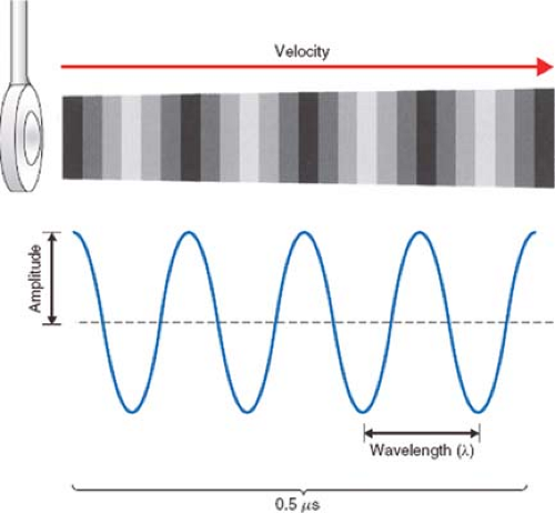 Figure 26.1. Sound wave. Vibrations of the ultrasound transducer create cycles of compression and rarefaction in the adjacent tissue. The ultrasound energy is characterized by its amplitude, wavelength, frequency, and propagation velocity. In this example, four sound waves are shown in a period of 0.5 μs. The frequency can be calculated as four cycles divided by 0.5 μs and equals 8 MHz. |
Properties of Sound Transmission in Tissue
The propagation of a sound wave through the body is markedly affected by its interactions with the various tissues encountered. These interactions result in reflection, refraction, scattering, and attenuation of the ultrasound signal and determine the resulting appearance of the two-dimensional image.
Echocardiographic imaging relies on the transmission and subsequent reflection of ultrasound energy back to the transducer. A sound wave propagates smoothly through uniform tissue until it encounters the interface between two tissues varying in acoustic impedance (a property largely related to the density [ρ] of the tissue and the speed that ultrasound travels). A large interface oriented perpendicular to the sound beam will produce a mirror-like reflection of sound back toward the transducer with only a portion of the signal passing through the interface. Since cardiac structures are detected by their reflected echocardiography signal, echocardiographers adjust the position of the TEE transducer so that the direction of its beam is perpendicular to the cardiac structure of interest.
Refraction causes a change in direction of propagating sound and occurs when an interface lies oblique to the sound beam. Refraction is an important factor in the formation of artifacts as the transducer mistakenly interprets a reflection from the refracted beam as originating from a cardiac structure located within the intended scanning field.
Scattering reflections occur when an ultrasound beam encounters small or irregularly shaped surfaces, such as red blood cells. These reflectors scatter ultrasound energy in all directions, so that far less energy is reflected back to the transducer. This type of reflection is the basis of the Doppler analysis of blood flow (see following).
Even when traveling through uniform tissue, sound undergoes a steady loss (i.e., attenuation) in intensity as a consequence of dispersion and absorption. Attenuation results in less energy returning to the transducer and low-quality images with poor signal-to-noise ratios. To combat attenuation, echocardiographers select better penetrating low-frequency signals (e.g., 2.5 instead of 7.5 MHz) and choose an imaging window that is close to the structure of interest. Adjusting the gain controls to amplify the weak returning signals makes their appearance brighter on the display. Unfortunately, this increases the brightness of artifactual noise, which negatively impacts the image appearance.
Instrumentation
Transducers
Ultrasound transducers use piezoelectric crystals to create a brief pulse of ultrasound. Alternating electrical current stimulates polarized particles within the crystal’s matrix to rapidly vibrate, generating ultrasound. Conversely, when a sound reflection strikes the crystal, the impact vibrates the polarized particles and generates an electric current. This property allows the piezoelectric crystal to function as both a transmitter and a receiver of ultrasound.
The shorter the length of the sound pulses, the better the axial resolution of the system. High-resolution imaging transducers emit sound pulses of just two to four cycles of short-wavelength, high-frequency sound.
Beam Shape
The ultrasound transducer emits a three-dimensional ultrasound beam similar to a movie projection (Fig. 26-2). The beam is narrow in the near field and then diverges into the far field zone. Focusing of the beam is used to improve spatial resolution by narrowing the ultrasound beam at the desired depth. The dense, narrow beam is preferred because it provides improved spatial resolution, produces high-intensity reflections, and reduces artifact. Echocardiographers adjust focal depth and focus to optimize the image resolution.
Resolution
Three parameters are evaluated when assessing the resolution of an ultrasound system: The resolution of objects lying along the axis of the ultrasound beam (axial resolution), the resolution of objects horizontal to the beam’s orientation (lateral resolution), and the resolution of objects lying vertical to the beam’s orientation (elevational resolution).
Short pulses of high-frequency ultrasound offer the greatest axial resolution but have a decreased tissue penetration. As resolution is highest along the axial plane, echocardiographic measurements are most precise when taken parallel to the beam’s axis. Accordingly, echocardiographers select transmitted frequency based on the particular imaging need.
Beam size determines the lateral and elevational resolution. Broad beams produce a “smeared” image of two nearby objects, whereas narrow beams can identify each object individually. Beam size is reduced by selecting high-signal frequencies and minimizing imaging depth.
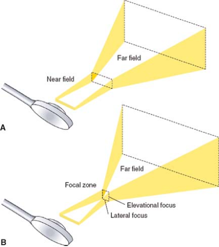 Figure 26.2. Three-dimensional beam. The ultrasound probe projects a three-dimensional beam. The dimensions of this projection have important effects on the imaging resolution and artifact. Typically, a narrow profile is preferred. A: Unfocused beam. The beam is narrow in the near field and then diverges in the far field. B: Focused beam. Focusing has resulted in a narrower beam in both the lateral and elevational planes, so that the imaging resolution of structures in the focal zone is improved. Distal to the focal zone, the beam rapidly diverges, and the images of structures in this area will be of lower quality. |
Signal Processing
To convert echoes into images, the returning ultrasound pulses are received, electronically processed, and displayed. The oscillator repeatedly cycles the transducer from a brief transmission to a relatively long receive mode. During the receive phase, the reflected echocardiography signals are captured and converted to electrical signals by the piezoelectric crystal. The echocardiography system employs a series of controls including system gain, time gain compensation, compression, and postprocessing settings (not unlike those available with digital imaging software) to optimize the signal for display. Adjustments are used, for example, to emphasize edge detection versus tissue texture, or to improve the delineation of weaker reflectors. The choice of settings is dictated by the examination and the preferences of the echocardiographer.
Image Display
Ultrasonic imaging is based on the amplitude and time delay of the reflected signals. Since the velocity in tissue is a relatively constant 1,540 m/s, only the distance of the structure from the transducer alters the time required for the ultrasound wave to travel to and from the reflected structure. So by timing the interval between transmission and return of the reflections, the echocardiography system can precisely calculate the distance of a structure from the transducer.
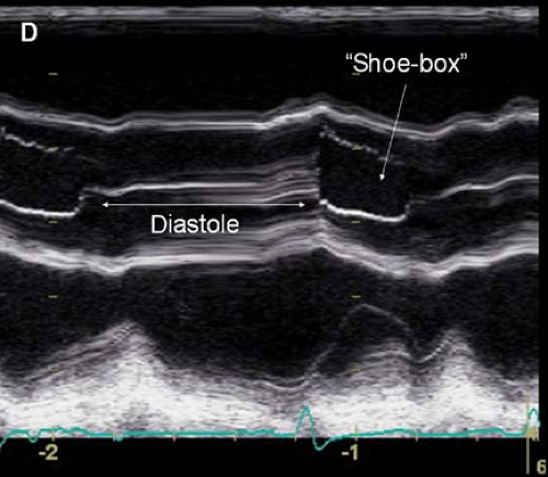 Figure 26.3. Method-mode (M-mode) echocardiography of a normal aortic valve. The M-mode cursor is placed at the center of the aortic valve and the motion of the aortic cusps over time is shown. During diastolic coaptation the aortic valve cusps appear as a thick, bright white line (long arrow), while in systolic apposition they form a “shoe-box” (short arrow). |
Current imaging is based on brightness mode or B-mode technology. With B-mode, the amplitude of the returning echoes from a single pulse determines the display brightness of the representative pixels. M-mode or motion mode adds temporal information to B-mode by displaying a series of sequentially collected B-mode images. M-mode echocardiography provides a one-dimensional, single-beam view through the heart but updates the B-mode images at a very high rate, providing dynamic real-time imaging. M-mode remains the best technique for examining the timing of cardiac events (Fig. 26-3).
Two-dimensional (2-D) echocardiography is a modification of B-mode echocardiography and the mainstay of the echocardiographic examination. Instead of repeatedly firing ultrasound pulses in a single direction, the transducer in 2-D echocardiography sequentially directs the ultrasound pulses across a sector of the cardiac anatomy. In this way, 2-D imaging displays a tomographic section of the cardiac anatomy, and unlike M-mode, reveals the shape and lateral motion (Fig. 26-4).
Two-dimensional scanning is achieved using phased array technology, which sequentially activates each crystal in the array and thereby steers the beam without the transducer itself being moved. The two commonly used electronic scanning systems in medical ultrasound are the linear scanners and sector scanners.
The linear scanner uses a long linear array. Groups of crystals are activated sequentially from one end of the transducer to the other. The firing of each group of crystals creates an image of the structures directly in front of them. With sequential firing, the anatomic features from one end of the transducer to the other are imaged (Fig. 26-5). The disadvantage of this approach is that the transducer face must be large to cover a broad anatomic area. The linear array is commonly used to guide vascular access and regional anesthetic procedures.
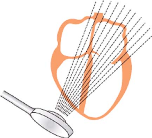 Figure 26.4. Scan lines. Illustration of the arced sector from a phased array two-dimensional echocardiogram. Each dotted line represents an individual brightness mode scan line. Any structure that interacts with a scan line will create reflections (dark highlight); however, structures that lie between the scan lines are not interrogated, and the echocardiography system averages the neighboring signals to fill in this defect. Accordingly, the closer the scan lines, the better the image quality. |
The phased array sector scanner is the most commonly used in echocardiography. Here the ultrasound scan is sequentially directed in a fan-like arc. The resulting sector image known as a frame is similar in shape to that covered by a windshield wiper. The 2-D scanner then repeats the entire process to update the image and capture motion.
Spatial Versus Dynamic Image Quality
Expert echocardiographers select machine settings to optimize particular image qualities for the examination at hand. As discussed in the following sections, these selections will determine whether sector size, spatial resolution, or dynamic motion is best displayed.
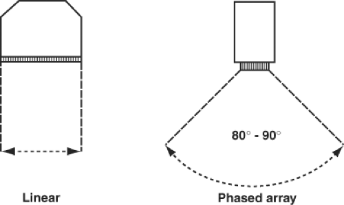 Figure 26.5. Linear scanners image a rectangular section of the anatomy compared with the arced sector imaged with phased array scanners. |
The pulse repetition frequency is the rate at which sound pulses are triggered. The greater the pulse repetition frequency, the greater the number of scan lines that are emitted in a given period of time. This enhances motion display. Unfortunately, sector depth must be reduced because pulse repetition frequency is inversely related to the sector depth as a longer period of time is required for the ultrasound to travel the increased distances.
The frame rate is the frequency at which the sector is rescanned. A high frame rate improves the capture of movement. Typically, frame rates >30 per second are desired. The frame rate is critically dependent on the sector depth, which determines the time required for each scan line to be received, and the sector width, which increases the number of scan lines that must be transmitted. Consequently, increases in sector size and depth come at the cost of a decreased frame rate and poor motion imaging.
The number of scan lines per degree of the sector (scan line density) greatly affects the image resolution. Doubling the scan lines essentially doubles the lateral resolution. However, the cost is a decrease in the frame rate and motion imaging.
The echocardiographer must thoughtfully select among settings that will often have opposing effects between the size of the imaging field, the imaging resolution, and the frame rate. A common approach is to focus each part of the examination on a given structure of interest and select the imaging plane that best delineates the structure in the near field. Motion display can then be enhanced without costs in lateral resolution by decreasing the sector angle and depth. In situations in which the maximal frame rate is desired, M-mode is chosen.
Two-Dimensional and Three-Dimensional Transesophageal Echocardiography Examination
TEE is the favored approach to intraoperative echocardiography. Compared with TTE, TEE offers additional “windows” to view the heart, often with improved image quality from the anatomic proximity of the esophagus and heart. In the operating room (OR), TEE is useful because the probe does not interfere with the operative field and can be left in situ, providing continuous, real-time hemodynamic information used to diagnose and manage critical cardiac events. TEE is also useful in situations in which the transthoracic examination is limited by various factors (obesity, emphysema, surgical dressings, and prosthetic valves) and for examining cardiac structures not well visualized with TTE (left atrial appendage).
This section is designed to introduce TEE image orientation and the diagnostic utility of each view. In addition, examination sequences useful for obtaining a comprehensive or targeted examination are provided. Readers are referred to A Practical Approach to Transesophageal Echocardiography.13 for a more detailed description of the TEE examinations described in this section.
Probe Insertion
resistance is encountered, additional force should be strictly avoided as oropharyngeal or esophageal injury may result. Rather, a decrease in neck extension and/or use of a laryngoscope to visualize the oropharyngeal structures often will allow easy passage of the probe. The TEE probe is advanced beyond the larynx and the cricopharyngeal muscle (around 25 to 30 cm from teeth) until a loss of resistance is appreciated. At this point, the TEE probe lies in the upper esophagus and the first cardiovascular images are seen. Extrinsic compression of the esophagus (e.g., osteophytes or an aortic aneurysm) may impede probe placement.9,10
Transesophageal Echocardiography Safety
TEE is a semi-invasive procedure. When performed by qualified operators, TEE has a low incidence of complications. A retrospective study performed on 846 patients who underwent TEE described the following complications: Three patients with pharyngeal abrasions, one patient with a chipped tooth, and few patients with transient vocal cord paresis.14 Another retrospective study performed on a large case series of 7,200 patients showed that the morbidity associated with TEE placement is 0.2% and the mortality is 0%.15 The most common complaint (0.1%) was postoperative odynophagia. Various studies have suggested an association between swallowing dysfunction after cardiac surgery and the use of intraoperative TEE.16,17 This fact is important as postoperative swallowing dysfunction is associated with pulmonary complications.16
Contraindication to Transesophageal Echocardiography Probe Placement
To maintain the safety profile of TEE, each patient should be evaluated before the procedure for signs, symptoms, or history of esophageal pathology. Amongst the most feared complications of TEE are esophageal or gastric perforation.18 For skilled practitioners, this complication is extremely rare. Patients with extensive esophageal and gastric diseases are at highest risk of perforation. Contraindications to TEE probe placement are represented by esophageal stricture, rings or webs, esophageal masses (especially malignant tumors), recent bleeding of esophageal varices, Zenker’s diverticulum, status post radiation to the neck, and recent gastric bypass surgery.13,18 In the rare case in which TEE is essential and is the only alternative, placement of the TEE probe can be performed under direct visualization with a combined gastroscopic and echocardiographic examination.13
Probe Manipulation
Image acquisition depends on precise manipulation of the TEE probe. By advancing the shaft of the probe, the probe position can be moved from the upper esophagus to the midesophagus and into the stomach. The shaft can also be manually rotated to the left or to the right. By using the large knob on the probe handle, the head of the probe can be anteflexed (turning the knob clockwise) and retroflexed (turning the knob counter clockwise). The smaller knob, located on top of the large knob, is used to tilt the head of the probe to the right or to the left. Using the electronic switch on the probe handle, the operator can rotate the ultrasound beam from 0 (transverse plane) to 180 degrees in 1-degree increments.
Orientation
The previously mentioned controls allow the experienced echocardiographers to perform comprehensive cardiac imaging. However, the diversity of imaging planes can confuse the less experienced echocardiographers, leaving them unable to recognize the various anatomic structures presented. Thus, an understanding of the basic rules of imaging orientation is essential to echocardiographic interpretation.
The ultrasound beam is always directed perpendicular to the probe face. The 2-D TEE image is displayed as a sector scan. The apex of the sector is in close proximity to the TEE probe and the structures seen in this area will be the posterior ones (e.g., left atrium). The arc of the sector will display the more distal and thereby more anterior structures. The angle of rotation of the imaging array determines the right and left orientations. An easy way to understand this orientation is to place your right hand in front of your chest with the palm facing down, the thumb oriented left and the fingers oriented anterior right. The scan lines that generate the TEE image start at your fingers and sweep toward the thumb. Consequently, the right anatomic structures will be displayed on the left side of the monitor (similar to chest x-ray orientation; Fig. 26-6). Increasing the imaging plane angle produces clockwise rotation of the sector scan. This can be visualized by rotating your hand in a clockwise fashion. For example, at the 90-degree imaging plane the left side of the screen now displays posterior structures (note position of fingers) and the right side of the screen anterior structures (note the position of the thumb; Fig. 26-7).
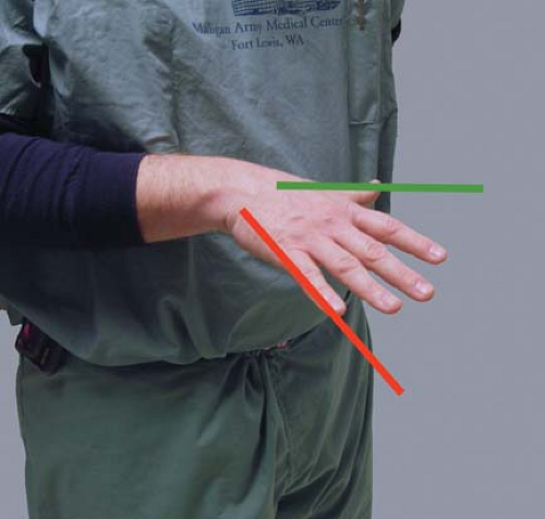 Figure 26.6. Orientation of the hand, as described in the text, for an imaging plane of 0 degree. The imaging plane is projected like a wedge anteriorly through the heart. The image is created by multiple scan lines traveling back and forth from the patient’s left (green line) to the patient’s right (red line). The resulting image is displayed on the monitor as a sector with the green edge (green line) on the right side of the monitor and the red edge (red line) on the left. |
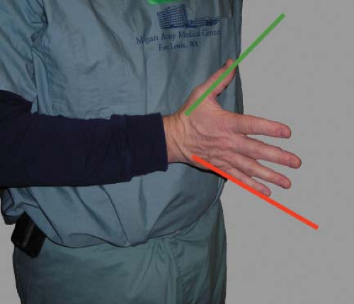 Figure 26.7. Orientation of the hand, as described in the text, for an imaging plane of 90 degrees. The imaging sector is rotated so that the green edge (green line) has moved clockwise and is now cephalad and the red edge is now caudad. As previously described, the green edge is displayed on the right side of the monitor and the red edge on the left. |
Goals of the Two-dimensional Examination
To achieve the goals of the intraoperative TEE examination, the Society of Cardiovascular Anesthesiologists together with the American Society of Echocardiography has published guidelines for performing a comprehensive intraoperative TEE examination.19 These guidelines include 20 standardized 2-D echocardiographic views. Each TEE examination should be recorded (video tapes or digital media) along with a detailed report of the examination. Miller et al.20 proposed a shortened version of the comprehensive examination that would meet the goals established by these guidelines for basic intraoperative TEE proficiency and is particularly useful when time constraints preclude a more extensive examination. The sequence in which the views are acquired differs among echocardiographers. In the following section, we detail the acquisition and anatomic features of the most commonly used intraoperative views.
 The midesophageal ascending aorta short-axis view.
This view is obtained by advancing the probe slightly from the upper esophagus until the ascending aorta (AA) is seen and then rotating the multiplane angle from 0 to 45 degrees to obtain a true short axis. This “great vessel view” images the AA in short axis and the main pulmonary artery (PA) with its bifurcation and right PA in long axis and the superior vena cava in short axis (Fig. 26-8). If the multiplane angle is advanced by ∼90 degrees, then the midesophageal AA long-axis view is obtained, in which the AA is visualized in a longitudinal cut and the right PA is visualized as a circular cross-sectional cut (Fig. 26-9). The main uses of the midesophageal ascending aorta short-axis view are to:
Measure the AA dimensions and evaluate the presence of dissection flaps
Evaluate the PA (position of catheter or rule out thrombus)
Align the Doppler beam parallel to the blood flow in the main PA
The midesophageal aortic valve short-axis view.
 This view is obtained from the previous view by advancing the probe until the aortic valve (AV) is visible, and then rotating the multiplane angle between 30 and 60 degrees. In
the closed position, the three cusps of the AV form what is known as the “Mercedes Benz” sign (Fig. 26-10). This view is used to:
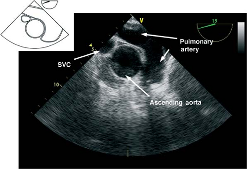
Figure 26.8. Midesophageal ascending aortic short-axis view. SVC, superior vena cava.
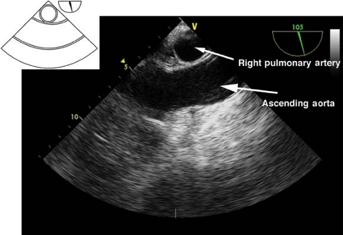
Figure 26.9. Midesophageal ascending aortic long-axis view.
Evaluate the size, number, appearance and motion of AV cusps
Measure the area of the AV orifice (planimetry)
Evaluate the presence of aortic insufficiency (AI) or aortic stenosis (AS) by applying color flow Doppler (CFD)
Assess the interatrial septum for patent foramen ovale (PFO) or atrial septal defect (ASD)
The midesophageal aortic valve long-axis view.
 This view is obtained from the previous view by rotating the multiplane angle to 120 to 160 degrees (Fig. 26-11). The view is used to assess:
The AV annulus, sinus of Valsalva, sinotubular junction, and AA dimensions
AI by using CFD
Vegetations or masses attached to the AV
Left ventricular outflow tract (LVOT) pathology (e.g., hypertrophic septum with possible LVOT obstruction)
The presence of calcification or dissection flaps in the proximal AA
The midesophageal bicaval view.
 This view is obtained from the previous view by turning the probe shaft to the patient’s right and decreasing the multiplane angle to ∼110 degrees (Fig. 26-12). The view is used to:
Assess the interatrial septum (aided by CFD) to detect a PFO or ASD. Evaluate the passage of agitated saline across the interatrial septum following release of a Valsalva maneuver
Guide placement of catheters, wires, and cannulae
Examine for the presence of thrombus or tumors
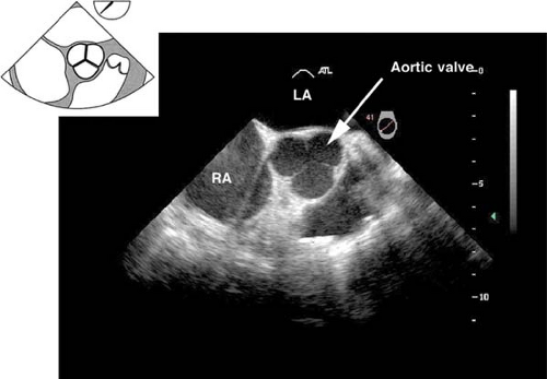
Figure 26.10. Midesophageal aortic valve short-axis view. RA, right atrium; LA, left atrium.
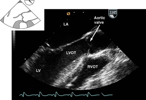
Figure 26.11. Midesophageal aortic valve long-axis view. LA, left atrium; LV, left ventricle; LVOT, left ventricular outflow tract; RVOT, right ventricular outflow tract.
 The midesophageal right ventricular inflow–outflow view. This view is obtained from the previous view by decreasing the multiplane angle to approximately 60 to 90 degrees (Fig. 26-13). The main uses of the view are to evaluate the:
Pulmonary valve (PV) by measuring the pulmonary annulus and to detect pulmonary insufficiency by applying CFD
RV and right ventricular outflow tract (RVOT) structure and function
Tricuspid valve (TV) anatomy and function by aligning the Doppler beam with the RV diastolic blood inflow or a systolic regurgitation
Passage of a PAC across the RV to the PA
 The midesophageal four-chamber view.
This view is obtained from the previous view by returning the multiplane angle between 0 and 20 degrees and slightly advancing the probe to the level of the mitral valve (MV). In this view, the four cardiac chambers and the TV and MV are visualized
(Fig. 26-14). Slight withdrawal or anteflexion of the probe will visualize the LVOT and AV and represents the midesophageal five-chamber view. The midesophageal four-chamber view is one of the most recognizable and valuable diagnostic views. Its main uses are to evaluate the:
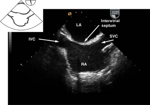
Figure 26.12. Midesophageal bicaval view. IVC, inferior vena cava; LA, left atrium; SVC, superior vena cava; RA, right atrium.
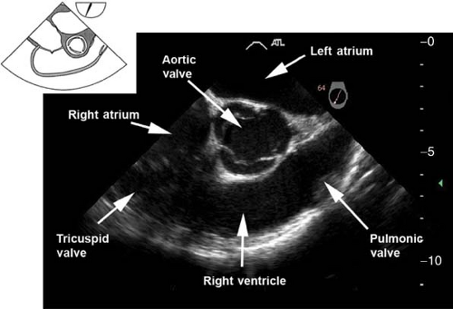
Figure 26.13. Midesophageal right ventricular inflow–outflow view.
Left atrium, right atrium, RV, and the LV (inferoseptal and anterolateral walls) size and function
TV and MV structure and function; CFD will detect valvular pathology
Diastolic function
The presence of atrial or ventricular septal defect
 The midesophageal two-chamber view.
This view is obtained from the previous view by rotating the multiplane angle to 90 degrees. In this view, the left atrial appendage is examined for the presence of thrombus. Slight retroflexion is used to avoid a foreshortened view of the LV so as to visualize the LV apex (Fig. 26-15). If the multiplane angle is rotated to just 60 degrees, then the midesophageal mitral commissural view is obtained (Fig. 26-16). The main uses of the midesophageal two-chamber view are to evaluate the:
 LV anterior and inferior wall function
LV apex as well as to diagnose apical thrombus
 The midesophageal long-axis view.
This view is obtained from the previous view by rotating the multiplane angle to 120 to 135 degrees (Fig. 26-17). The main uses of the midesophageal long-axis view are to evaluate the:
LV anteroseptal and posterior wall function
LV outflow tract pathology
MV anatomy and function
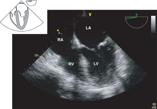
Figure 26.14. Midesophageal four-chamber view. RA, right atrium; RV, right ventricle; LA, left atrium; LV, left ventricle.
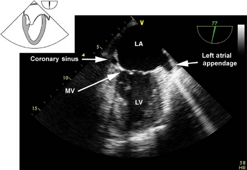
Figure 26.15. Midesophageal two-chamber view. LA, left atrium; MV, mitral valve; LV, left ventricle.
 The transgastric midpapillary short-axis view.
 The view is obtained by advancing the TEE probe from the midesophageal four-chamber view into the stomach, anteflexing and then withdrawing until contact is made with the gastric wall. The LV is visualized as a doughnut in cross-section and both papillary muscles should be seen (Fig. 26-18). Additional anteflexion obtains the transgastric basal short-axis view (Fig. 26-19), which allows for inspection of the anterior and posterior mitral valve leaflets. Advancement of the probe allows visualization of the LV apex in cross-section. The transgastric midpapillary short-axis view is unique in that it visualizes LV walls perfused by each of the three major coronary arteries. The view is considered to be the most useful one in situations of intraoperative hemodynamic instability as it allows immediate diagnosis of hypovolemic state, contractile failure, or coronary ischemia.
The primary uses of the transgastric midpapillary short-axis view include assessment of the:
LV size (enlargement, hypertrophy) and cavity volume
Global ventricular systolic function and regional wall motion
The transgastric two-chamber view.
 This view is obtained from the previous one by rotating the multiplane angle to 90 degrees. The LV is visualized in a longitudinal section with the apex at the left of the display and MV at the right (Fig. 26-20). The primary use of this view is to:
Assess function of the LV anterior and inferior walls
Evaluate the anatomy and function of the MV and chordae tendineae
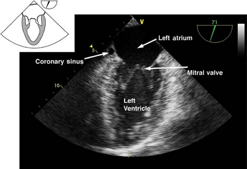
Figure 26.16. Midesophageal commissural view.
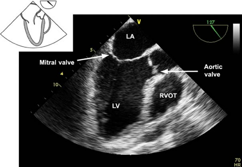
Figure 26.17. Midesophageal long-axis view. LA, left atrium; LV, left ventricle; RVOT, right ventricular outflow tract.
The transgastric long-axis view.
 This view is obtained from the previous view by rotating the multiplane angle to 120 degrees (Fig. 26-21). The main uses of the view are to:
Position the Doppler beam parallel to blood flow across the LVOT and AV
Assess systolic function of the anteroseptal and inferolateral LV walls
The deep transgastric long-axis view.
 This view is obtained by advancing the probe deep in the stomach, toward the LV apex, and then anteflexing and slightly withdrawing the probe (Fig. 26-22). The main use of the view is:
Doppler assessment of LVOT and aortic blood velocities
Evaluation of AV function with CFD
Descending aortic short- and long-axis views.
 The descending aortic short-axis view is obtained from the midesophageal four-chamber view by turning the TEE probe to the left until the descending aorta in cross-section is seen as a circular structure (Fig. 26-23). Rotating the multiplane angle to 90 degrees visualizes the descending aorta in a longitudinal section as a tubular vascular structure (Fig. 26-24).
In order to examine the entire descending aorta, the probe is gradually advanced and withdrawn in the esophagus. These views are used to:
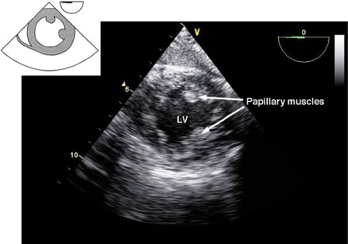
Figure 26.18. Transgastric short-axis view. LV, left ventricle.
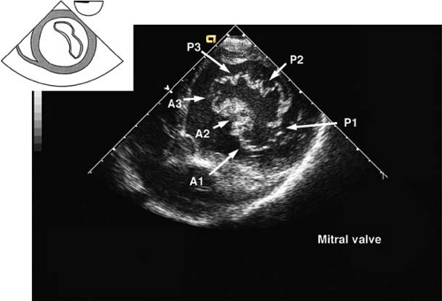
Figure 26.19. Transgastric basal short-axis view. A1–3, anterior leaflet of mitral valve, scallops 1–3; P1–3, posterior leaflet of mitral valve, scallops 1–3.
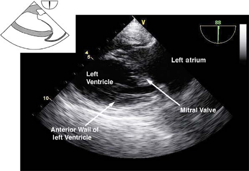
Figure 26.20. Transgastric two-chamber view.
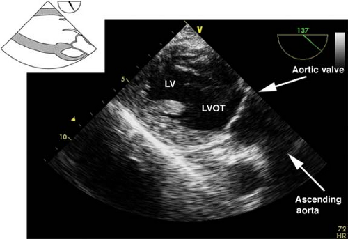
Figure 26.21. Transgastric long-axis view. LV, left ventricle; LVOT, left ventricular outflow tract.
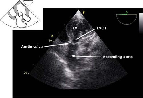
Figure 26.22. Deep transgastric long-axis view. LV, left ventricle; LVOT, left ventricular outflow tract.
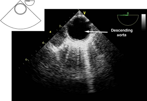
Figure 26.23. Descending aortic short-axis view.
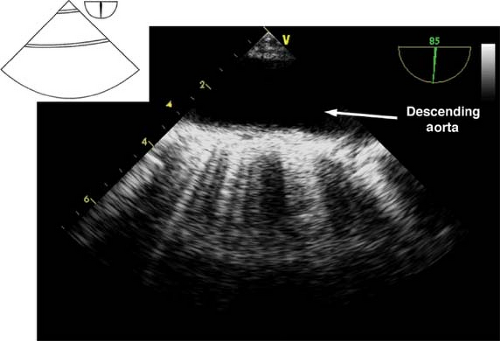
Figure 26.24. Descending aortic long-axis view.
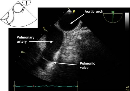
Figure 26.25. Upper esophageal aortic arch short-axis view.
Identify pathology of the descending aorta (atheroma, hematoma, dissection flaps, aneurysm)
Assist with placement of guide wires and cannulae (intra-aortic balloon pump [IABP], aortic cannula)
 Upper esophageal aortic arch short-axis view.
 The view is obtained from the descending aortic long-axis view by withdrawing the probe in the upper esophagus and turning it to the right until the tubular structure transforms into a circular one (Fig. 26-25). The view is used to assess the presence of pathology in the distal aortic arch and Doppler assessment of pulmonary artery blood velocities. If the multiplane angle is rotated back to 0 degree, the upper esophageal aortic arch long-axis view is obtained (Fig. 26-26).
Three-dimensional Echocardiography
In order to better conceptualize the morphology and pathology of the heart, three-dimensional (3-D) image presentation has been developed. The recent introduction of a real-time 3-D TEE probe makes this goal a reality for intraoperative echocardiographers. This technology is capable of acquiring full volumes of the left ventricle, of visualizing heart valves in three dimensions (Fig. 26-27), and assessing the synchrony of LV contraction.21
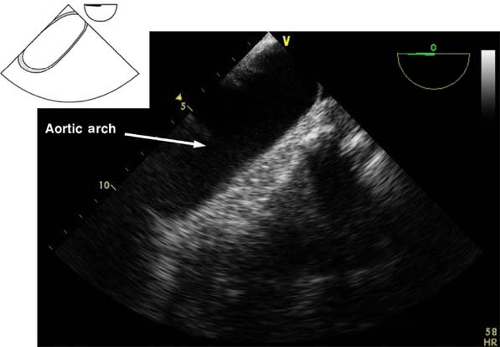 Figure 26.26. Upper esophageal aortic arch long-axis view. |
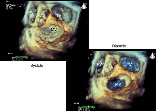 Figure 26.27. Three-dimensional transesophageal echocardiographic imaging of the base of the heart with the atria removed, in systole and diastole. AV, aortic valve; MV, mitral valve; PV, pulmonic valve; TV, tricuspid valve. |
Uses of 3-D TEE are just emerging. The utility of 3-D imaging of the MV for an MV repair surgery is of particular interest (Fig. 26-28).22 The capacity of this probe to assess LV contraction synchrony in patients undergoing resynchronization therapy with biventricular pacing may offer a means to maximize their cardiac output. Additional intraoperative applications have emerged, involving percutaneous procedures (transcutaneous aortic valve insertion, noninvasive mitral repair, repair of paraprosthetic leaks, closure of ASD) and open surgical procedures. Guidelines on the use of 3-D echocardiography have also been published.23
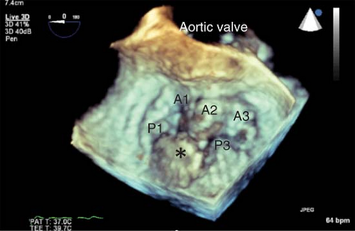 Figure 26.28. Three-dimensional imaging of prolapsing middle scallop of the posterior mitral valve leaflet (asterisk). A1–3, lateral, middle and medial scallops of the anterior mitral valve leaflet; P1, lateral scallop of the posterior mitral valve leaflet; P3, medial scallop of the posterior mitral valve leaflet. |
Doppler Echocardiography and Hemodynamics
The motion of an object causes a sound wave to be compressed in the direction of the motion and expanded in the direction opposite to the motion. This alteration in frequency is known as the Doppler effect. By monitoring the frequency pattern of reflections of red blood cells, Doppler echocardiography can determine the speed, direction, and timing of blood flow. The Doppler equation describes the relationship between the alteration in ultrasound frequency and blood flow velocity (Fig. 26-29)
where Δf is the difference between transmitted frequency (ft) and received frequency, v is blood velocity, c is the speed of sound in blood (1,540 m/s), and θ is the angle of incidence between the ultrasound beam and blood flow. Conceptually, the equation is simplified by observing that the change in ultrasound frequency is related to just two variables: Blood velocity and cos θ. For this reason the Doppler signal is shifted only by the component of the blood velocity that is in the direction of the beam path (i.e., v cos θ).
When the beam angle divergence is >30 degrees the value of cos θ decreases rapidly and the Doppler system will markedly underestimate blood velocity. The requirement of near-parallel orientation (cos 0 = 1) for Doppler examinations contrasts with the near-perpendicular orientation preferred for 2-D imaging. Consequently, the preferred imaging planes for Doppler will differ from those used for 2-D imaging.
When the beam angle divergence is >30 degrees the value of cos θ decreases rapidly and the Doppler system will markedly underestimate blood velocity. The requirement of near-parallel orientation (cos 0 = 1) for Doppler examinations contrasts with the near-perpendicular orientation preferred for 2-D imaging. Consequently, the preferred imaging planes for Doppler will differ from those used for 2-D imaging.
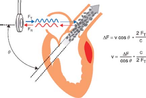 Figure 26.29. Calculating blood flow velocity: The Doppler equation. The Doppler equation calculates blood flow velocity based on two variables: The Doppler frequency shift (ΔF) and the cosine (cos) of the angle of incidence between the ultrasound beam and the blood flow. The Doppler frequency shift is measured by the echocardiographic system, but cos θ is unknown, and manual entry by the echocardiographer is required for its estimation. v, flood flow velocity; FT, transmitted signal frequency; FR, reflected signal frequency; ΔF, difference between FR, and FT; c, speed of sound in tissue; θ, angle of incidence between the orientation of the ultrasound beam and that of the blood flow. |
Spectral Doppler
Two Doppler techniques, pulsed wave (PW) and continuous wave (CW), are commonly used to evaluate blood flow. A thorough understanding of the advantages and disadvantages of each technique is critical in selecting the one most appropriate for the clinical setting at hand.25,26 In clinical practice, PW and CW Dopplers are frequently used in conjunction with 2-D imaging. The 2-D image is used to identify the area of interest and guide the echocardiographer in precisely localizing the sampling volume in a PW study or in directing the beam in a CW study.
Pulsed-wave Doppler
PW Doppler offers the echocardiographer the ability to sample blood flow velocity from a particular location. The PW transducer uses a single crystal as both the emitter and the receiver of ultrasound waves. Like the pulsed echocardiography system described for 2-D imaging, the PW Doppler system transmits a short burst of ultrasound toward the target and then switches to receive mode to interpret the returning echoes. Since the speed of sound (c) in tissue is constant, the time delay for a signal to reach its target and return to the transducer depends solely on the distance (d) to the target. Consequently, reflected signals from locations more distant from the transducer return after a greater time interval. By time gating, the electronic circuitry of the PW transducer interprets returning echoes only after a predetermined time delay following the transmission of an ultrasound pulse. In this way, only those signals associated with a location, referred to as the sample volume, are selected for evaluation.
The pulsed-Doppler system uses a repeating pattern of ultrasound transmission and reception. The rate at which the device repeatedly generates sound bursts is known as the pulse repetition frequency. Since the speed of sound through tissue is a constant, the pulse repetition frequency is directly related to the depth of the sample volume. The pulse repetition frequency is analogous to the frame rate of a movie camera. Like the multiple frames on a roll of movie film, each ultrasound pulse interacts with the blood flow for a brief period of time, and just as a series of movie frames display motion, a series of pulsed cycles are consecutively analyzed to determine the blood flow. The Doppler data is frequently presented as a velocity–time plot known as the spectral display (Fig. 26-30B).
Since the pulsed-Doppler data are collected intermittently, the maximal frequency and blood flow velocity that can be accurately measured by PW Doppler are limited. The maximal frequency, which equals one-half the pulse repetition frequency, is known as the Nyquist limit. At blood velocities above the Nyquist limit, analysis of the returning signal becomes ambiguous, with the velocities appearing to be in the opposite direction. A similar effect is seen in movie animation, in which a rapidly spinning wheel appears to spin backward because of the slow frame rate. The ambiguous signal from frequencies above the Nyquist limit produces aliasing, and the velocity signal may appear on the other side of the zero velocity baseline, hence the term wraparound. The Nyquist limitation has led to an alternative approach for the assessment of high-velocity blood flows, namely CW Doppler.
Continuous-wave Doppler
The CW Doppler technique avoids the maximal velocity limitation of PW systems by using two crystals, one continuously transmitting and the other continuously receiving the reflected ultrasound signal. With continuous reception of the Doppler signal, the Nyquist limit is not applicable, and blood flows with very high velocities are recorded accurately. The CW mode receives reflected signals from blood flow throughout its beam path because it is not time-gated like the PW technique (Fig. 26-30A). The inability to select blood flow from a specific location favors the selection of CW Doppler primarily for the detection of the highest velocities along the beam path, which is useful in applications such as determining the high velocity jet of aortic stenosis.
Color-flow Doppler
CFD provides a dramatic display of both blood flow and cardiac anatomy by combining 2-D echocardiography and Doppler (Fig. 26-31). The PW Doppler used for CFD differs from that previously discussed in two important ways. CFD performs multiple sample volume recordings along each scan line as the beam is swept through the sector. This approach provides flow data at each location in the sector, which can be overlaid on the structural data obtained by 2-D imaging. The Doppler velocity data from each sample volume are color-coded and superimposed on top of the gray scale 2-D image. In the most widely accepted color code, red hues indicate flow toward the transducer and blue hues indicates flow away from the transducer. The ability to provide a real-time, integrated display of flow and structural information makes CFD useful for assessing valvular function, aortic dissection, and congenital heart abnormalities. However, an important caveat to its use in the clinical setting must be noted. Since it relies on PW Doppler measurements, CFD is susceptible to alias artifacts. Aliasing in the color flow map is illustrated in Figure 26-32. This alias pattern
can be useful to calculate blood flow in mitral valve disease using the proximal isovelocity surface area (PISA) method (Fig. 26-32).
can be useful to calculate blood flow in mitral valve disease using the proximal isovelocity surface area (PISA) method (Fig. 26-32).
Related posts:


Stay updated, free articles. Join our Telegram channel

Full access? Get Clinical Tree


