The measurement system as a ‘black box’
The measurement system in turn consists of component ‘black boxes’ representing:
A transducer – a detecting element which converts the quantity being measured (the input) into usable data or a signal, usually an electrical signal. Examples of common transducers are:
a microphone, which converts sound to an electrical signal
a thermistor, which converts temperature variations into an electrical signal
a piezoelectric crystal, which converts pressure variations into an electrical signal
A transmission path – this is the means by which the transducer signal is transferred to the signal conditioning unit or the display unit. Examples include electrical or optic cables, a length of tubing or an infrared link.
A signal conditioning unit – this processes the transducer signal in order to make it suitable for display or storage. Signal processing includes functions such as amplification, filtering, and analogue to digital conversion. It may occur before or after the signal passes along the transmission path.
A display and/or storage unit – this provides the output of the system as a display and also stores the signals or data. It may employ analogue or digital methods. Sometimes a distinction is drawn between a system displaying a signal (e.g. capnograph) as opposed to a numerical value (e.g. capnometer). Some examples are given in Figure 45.2.
| Function | Analogue | Digital |
|---|---|---|
| Display | Oscilloscope Moving coil meter Chart recorder | Digital voltmeter Light-emitting diodes Liquid crystal display |
| Storage | Magnetic tape Chart | Computer hard disk Floppy disc Magnetic tape CD-ROM USB flash drive |
Characteristics of a measurement system
The performance of a measurement system is characterised by its static and dynamic characteristics. These determine the relationship between the quantity being measured (input) and the measurement (output).
Static characteristics define the performance of a measurement system when dealing with an input that is not changing or only changing slowly. Under these circumstances there is enough time for the system to reach a steady state before the measured quantity changes, so that the output follows changes in the input accurately.
The dynamic characteristics of a system reflect its ability to respond to rapidly changing inputs. Every system requires a certain time to settle to a steady state when presented with a change in its input. This response time may affect the accuracy of the measurement, since if the input is changing rapidly, the measuring system may not have adequate time to reach steady state and thus will not give an accurate reading.
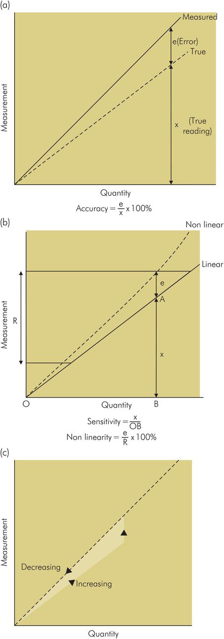
Static characteristics
Accuracy – This refers to the closeness between the measurement obtained and the ‘true’ value of the quantity being measured. For example, if a pressure has a ‘true’ value of 10 cmH2O, an accurate system may read 10.01 cmH2O and may be described as having an accuracy of 0.1%. In an inaccurate system reading 11 cmH2O the accuracy may be quoted as 10% (Figure 45.3a).
Sensitivity – This is the relationship between changes in the output reading of the system and changes in the measured quantity. The sensitivity of a pressure measurement system may be described as the change in output signal voltage for a given change in pressure, e.g. 1 volt per cmH2O for a sensitive system or 100 millivolts per cmH2O for a system 10 times less sensitive. Less sensitive systems will cover a wider range of pressure measurement than sensitive systems (Figure 45.3b).
Linearity – In a linear measurement system the output reading varies in proportion to the measured quantity. Thus in a linear pressure measurement system, if the pressure doubles the output voltage will double. When the output voltage is plotted against the input pressure, a straight line is obtained. The gradient of this line gives the sensitivity of the system. It is usually desirable for a system to be linear, and any non-linearity is quoted as a percentage of the operating range of the instrument (Figure 45.3b). Some instruments may be intrinsically non-linear, reflecting their underlying mechanism – e.g. hot wire ammeter, rotameter.
Hysteresis – This is a property of a measurement system which produces an error dependent on whether the measured value is decreasing or increasing. Hysteresis in a mechanical device is caused by elastic energy stored in the system, or frictional losses and slack movement of moving parts. Figure 45.3c shows how hysteresis in a measurement system produces errors in the measurement of increasing and decreasing pressures.
Drift – This is variation in the reading from an instrument which is not caused by change in the measured quantity. It is usually caused by the effect of internal or external temperature changes on the measurement system, and unstable components in the system.
Dynamic characteristics
Step response
An important dynamic characteristic of any measurement system is its response to a rapid increase in input or a ‘step’ function (Figure 45.4). This can be simulated by dipping a thermometer at room temperature into boiling water, or rapidly opening a tap connecting a pressure gauge to a pressurised container. In a perfect measuring instrument, the output or ‘step response’ produced by a step input should also be a step function, occurring instantaneously to give a reading of the measured quantity.
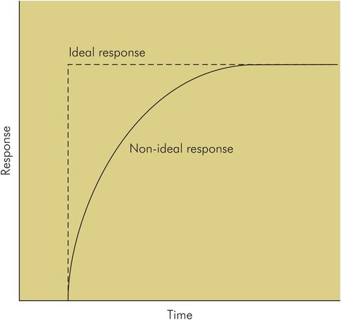
Ideal and non-ideal step responses of a measurement system
In practice, the step response differs from the ideal due to the properties of the system, and the output only reaches a ‘true’ steady state value after a finite time. The time lag for an instrument between a step input and the output reaching its final value is reflected by:
Response time – the time taken from occurrence of the step input to the instrument output reaching 90% of its final value
Rise time – the time taken for the output of the instrument to rise from 10% to 90% of its final value (Figure 45.4)
Damping
The step response of an instrument may also fall short of the ideal in the shape of the output signal produced. Some examples are shown in Figure 45.5. In response curve (a), under-damped, the output overshoots and oscillates about the true value; in curve (b), over-damped, the response does not reach the true value in the time plotted; and in curve (c), critical damping, the output reaches a steady reading of the true value within a short time with no overshoot. The property which determines the nature of the step response is called the damping of the system.
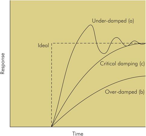
Damping is an important factor in the design of any system. In a measurement system it can lead to inaccuracy of the readings or display.
Under-damping can result in oscillation and overestimation of the measurement.
Over-damping can result in underestimation of the measurement.
Critical damping is usually an optimum compromise resulting in the fastest steady-state reading for a particular system, with no overshoot or oscillation.
All instruments will possess damping, which affects their dynamic response. This includes mechanical, hydraulic, pneumatic and electrical devices. In an electromechanical device such as a galvonometer there are mechanical moving parts such as the meter needle and bearings. Damping in these components arises from frictional effects on their movement. This may arise unintentionally or may be applied as part of the instrument design to control oscillation of the needle when it records a measurement. In a fluid (gas or liquid)-operated device damping occurs because of viscous forces which oppose the motion of the fluid, while in electrical systems damping is provided electronically by electrical resistance which opposes the passage of electrical currents.
Frequency response
Any measurement system in practice will only respond to a restricted range of frequencies, either by design or due to the limitations of its components. If the system were to be tested with input signals of the same amplitude but different frequencies it would only produce an output over a limited range of frequencies. Within this frequency range the system may respond more sensitively to some frequencies than others. When the system response is plotted against signal frequency the resultant curve is called the frequency response of the system (Figure 45.6).
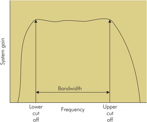
Frequency response of a system to an input signal with constant amplitude but at different frequencies
Bandwidth
The highest frequency that a system responds to is the high cutoff frequency, above which input signals will produce no output. An example of such a cutoff is in the frequency response of the human auditory system, which at best may have a high cutoff frequency of 20 kHz. Similarly a system may possess a low cutoff frequency, the lowest frequency audible by the human ear being 15 Hz. The frequency range between low and high cutoff frequencies, is referred to as the bandwidth, which in the human ear is 19.985 kHz.
Distortion due to poor frequency response
Any input signal can be characterised by its frequency spectrum (see below), which defines the different frequency components into which the signal can be resolved. Distortion may occur if the frequency response of a measurement system does not cover the spectrum of a signal, thus blocking part of the input signal. Alternatively, an instrument may be more sensitive to certain frequencies and enhance or attenuate them, causing it to give falsely high or low readings within its operating frequency range. This can occur at natural frequencies or resonances and anti-resonances (see below). Distortion due to poor frequency response of a system is illustrated in Figure 45.7.
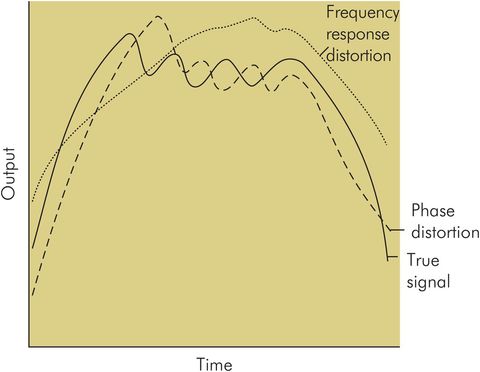
Signal distortion due to poor frequency response and phase response
It might initially be assumed that the ideal frequency response for a system would be one with equal sensitivity at all frequencies, from very low to very high (i.e. a flat response from 0 to ∞ Hz), but this would also enable ‘noise’ to pass through the system with the measurement signal, causing error and distortion.
The frequency response of a mechanical system is determined by its inertial and compliance elements (equivalent to masses and springs), while in an electrical circuit it is determined by the inductances and capacitances. There is often a design compromise between providing accuracy and reducing noise levels.
Natural frequencies or resonances
A measurement system may possess natural frequencies or resonances determined by inertial and compliance elements in a mechanical system (or inductances and capacitances in an electrical circuit). These resonances appear as peaks in the system’s frequency response and can produce distortion in a signal display and errors in the readings (Figure 45.8). Good design practice can ensure that these resonances do not lie in the operating frequency range of the instrument, or can use appropriate levels of damping to smooth out these unwanted peaks in an instrument’s frequency response.
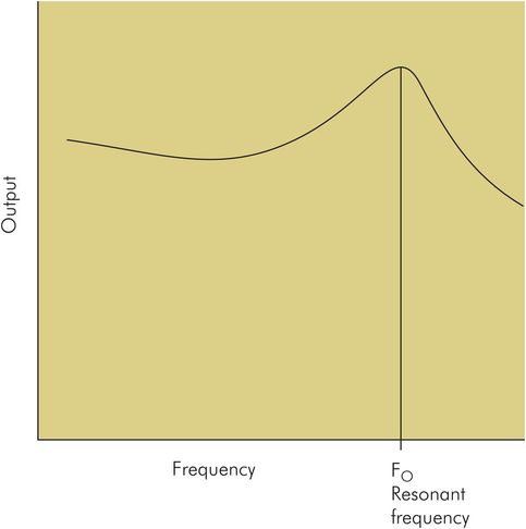
Resonant frequency response
Phase shift response
Fourier analysis demonstrates how a signal is composed of a series of component frequencies. In a signal being processed, each frequency component will undergo a different delay in time or phase shift as it passes through the measurement system (a phase shift is a time delay expressed as an angle, i.e. the units are degrees or radians – see Phase angle, under Electric circuits in Chapter 44). If the relative phases between frequency components of a signal are altered too much, distortion of the signal occurs and inaccuracy is introduced. Any measurement system will have a phase shift response, consisting of the phase shift occurring at different frequencies, which can be plotted against the frequency axis. In a simple system at resonant frequency the phase shift will be 90°. This phase shift response will be dependent on the components of the system, and can be responsible for distortion or errors in an instrument (Figure 45.7).
Electrical signals
In modern measuring instruments the transducer usually produces an electrical current or voltage, which varies according to the measured parameter. This voltage or current is a signal. Signals in clinical measurement are usually voltage signals or biological potentials. Most biological potentials vary in time, many in a repetitive or cyclical fashion – e.g. electrocardiogram, airway pressure during respiration. Some signals, such as the electroencephalogram and evoked potentials, are not cyclical but vary irregularly.
Biological potentials
The characteristics of some common biological potentials are outlined in Figure 45.9.
| Signal | Voltage range | Frequency range (Hz) |
|---|---|---|
| Electroencephalogram (EEG) | 1–500 μV | 0–60 |
| Electrocardiogram (ECG) | 0.1–50 mV | 0–100 |
| Electromyogram (EMG) | 0.01–100 mV | 0–1000 |
Characteristics of electrical signals
Electrical signals can be described in the following ways:
As a voltage (or current) varying in time – The amplitude of a signal is the range of variation between maximum and minimum values (Figure 45.10).
As periodic or non-periodic – A signal which varies with a repeating pattern in time, at regular intervals, is said to be periodic. The simplest type of periodic signal is a sine wave (Figure 45.10).
As analogue or digital – An analogue signal is continuous in time and the magnitude of the signal varies smoothly without discernible increments. A digital signal is produced from an analogue signal by sampling the signal at regular intervals, and can be represented by a set of numbers. This adapts the signal for processing by digital systems and manipulation by computer (Figure 45.11).
As a series of frequency components – A mathematical method of analysis was invented by Baron de Fourier in 1822. This has evolved both theoretically and practically to become one of the most powerful tools used in signal processing. Application of Fourier analysis to a signal enables it to be described by its frequency spectrum.
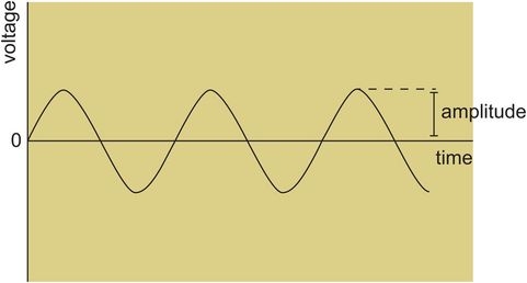
Periodic signal plotted against time – sine wave
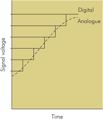
Analogue and digital signal
Frequency spectrum of a signal
The description of a signal by its frequency spectrum can be summarised by:
Any signal varying continuously in time can be broken down into a collection of sine and cosine waves, which if added together yield the original signal.
The component waves exist as sine–cosine pairs at the same frequency.
Each pair of components has a combined amplitude and can be plotted as a point on the frequency axis, giving the frequency spectrum for the signal.
Conversion of a signal into its frequency components is referred to as spectral analysis or Fourier analysis. Fourier analysis is most suitable for periodic wave forms, but can still be used for non-periodic wave forms using an approximation (or mathematical ‘trick’) which treats the waveform as if it were a periodic signal with a very long period.
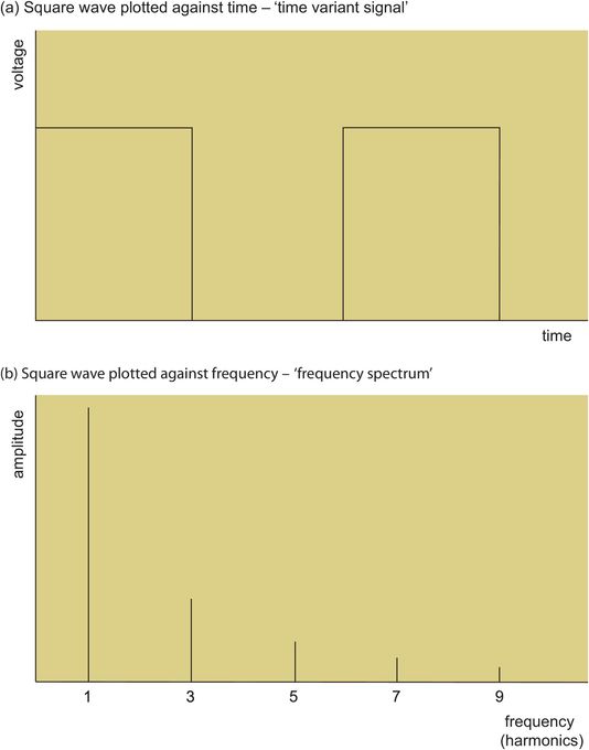
Figure 45.12a shows a square-wave signal plotted against the time axis as a time-variant periodic signal. It can also be plotted against the frequency axis as a series of frequency components or harmonics (Figure 45.12b). This gives an approximation to the frequency spectrum of the square wave. The frequency spectrum of a signal is related to the shape of its waveform. In general the more ‘spiky’ and ‘pointed’ the waveform, the higher the range of component frequencies contained.
Electrical ‘noise’
A signal may be modified by any of the components of the measurement system. If the changes introduced are intentional, they represent signal processing or signal conditioning. Unwanted alteration of the signal by the system is distortion and introduces error.
Noise can change the amplitude of a signal and alter its appearance on display, causing inaccuracy. Noise signals may be generated by the components of the measurement system itself, or may be picked up as interference from external sources such as diathermy or fluorescent lighting.
Signal-to-noise ratio
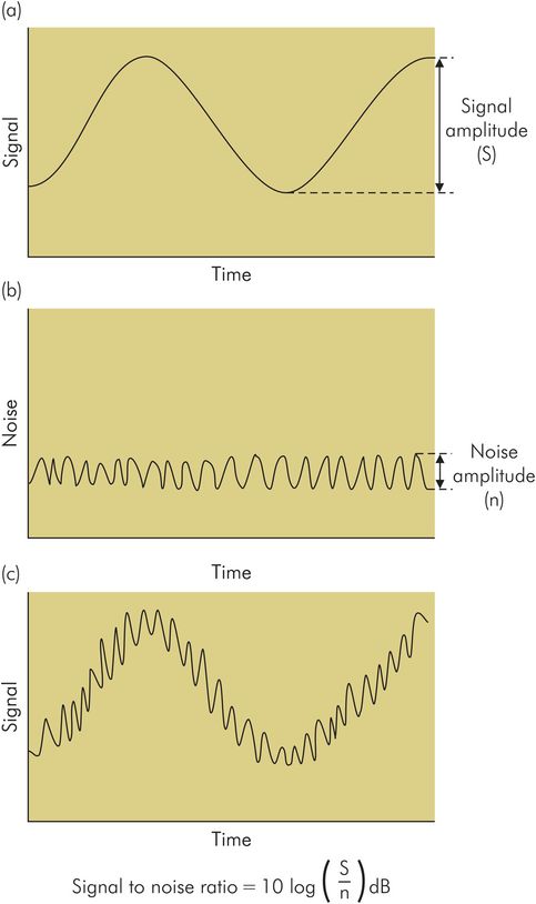
In some cases the noise signals may be so large as to obscure the measurement signal altogether. An awareness of the magnitude of noise components in the signal is necessary in order to assess the accuracy of the measurements. This can be expressed by the signal-to-noise (S/N) ratio.
Electrical ‘noise’ is an unwanted component added to the signal by the signal processing system or due to outside electrical interference.
The signal-to-noise (S/N) ratio is the ratio of signal amplitude to noise amplitude expressed in decibels (Figure 45.13).
Signal processing
Signal processing improves a raw signal by:
Amplification – Many biological signals are very small in amplitude (e.g. EEG signals may only be in microvolts, while ECG signals may only be in millivolts). Such signals are usually too small to drive display or storage units, and require amplification. Low-amplitude signals are also unsuitable for transmission, since noise signals picked up may be of similar or greater amplitude, giving a low S/N ratio and obscuring the signal.
Filtering to remove noise – Often noise signals are in a different frequency range from the wanted measurement signal. In these cases the noise can be reduced by using filters to block out the unwanted frequencies:
A low pass filter rejects all frequencies above a given threshold. Such a filter would be used to avoid high frequency interference from a source like diathermy.
A high pass filter rejects low frequencies below a set threshold.
A notch filter rejects a specific frequency such as 50 Hz to avoid pick-up from mains cables.
Spectral analysis – A signal is usually displayed as a time-varying voltage or currrent. In some cases (e.g. cerebral function monitoring) a display of the signal frequency spectrum is required, which can be achieved using electronic processing. A common method first converts the analogue signal to a digital signal, and then applies a mathematical algorithm called the Fast Fourier Transform (FFT). Transformation of a signal to its spectral components can also make some processing functions such as filtering easier and more accurate, and it also enables more complex analysis to be readily performed by computers.
Analogue to digital (A to D) conversion – This conversion is often required before applying other processing functions, and is always necessary in order for the signal to be stored and analysed in a computer. This is because most electronic manipulation of signals uses digital electronics as opposed to analogue methods.
Averaging to remove noise – In some cases the amplitude of the measurement signal may only be a fraction of the noise amplitude (i.e. the S/N ratio is very low). In such a case, the wanted signal may be completely obscured by noise. If the wanted signal is repetitive and the noise is random in time, multiple repetitions and summations of the noisy signal lead to an increase of the S/N ratio as the random noise cancels itself out. This is called averaging and is used in the extraction of evoked potentials, where the evoked signal is only a few millivolts in amplitude, hidden in background noise (EEG signals and neuromuscular activity). Averaging over 2000 or more repetitions may be required to obtain a clear signal.
Amplifiers
An amplifier is an electronic ‘black box’ which increases the amplitude of an electrical signal fed into its input. The purpose of an amplifier in measuring systems is to increase the power of a low-amplitude signal so that it can be used to drive a display or storage unit. The amplifier requires a power supply, and it channels power from this power supply into the input signal, increasing its voltage and current levels.
Characteristics of an amplifier include:
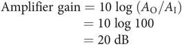
Gain – this is the ratio of the amplitude of the output signal (AO) to the input signal (AI). It is usually expressed in decibels (dB – these units may be used to express any ratio by taking 10 times the log10 of the ratio).
Frequency response and phase response – these are determined by the amplifier’s circuit design.
Upper cutoff frequency – this is the upper frequency limit above which signals are blocked or ‘cut off’. It is measured in hertz (Hz).
Lower cutoff frequency – this is the lower frequency limit below which signals are blocked or ‘cut off’.
Bandwidth – this is the extent of the frequency range passed by a system or amplifier: i.e. the amplifier only amplifies signals within this frequency range. It therefore lies between upper and lower cutoff frequencies and is also measured in frequency units (Hz).
Input impedance – this is the electrical impedance ‘seen’ by the transducer signal at the input of the amplifier. Maximum power transfer takes place when the input impedance of the amplifier matches the output impedance of the trandsducer. It is measured in ohms.
Output impedance – this is the electrical impedance seen ‘looking’ back into the output terminals of the amplifier. Maximum transfer of signal power from the amplifier requires matching of the output impedance to the input impedance of the transmission path or the display unit.
If the output amplitude produced by an amplifier, AO, is 100 times the input amplitude, AI:
Pressure measurement
Pressure is defined as force per unit area and is measured in various units in the clinical setting, depending on the quantity being measured. Some examples are shown in Figure 45.14.
| Quantity measured | Unit |
|---|---|
| Blood pressure | mmHg |
| Airway pressure | cmH2O |
| Partial pressure of blood gas | kPa |
| Gas cylinder pressure | bar, psi |
In anaesthesia, pressure measurements are usually made in gases (gas cylinders, anaesthetic machines, breathing circuits) or liquids (intra-arterial pressure monitoring).
Pressures are not usually absolute measurements but are generally measured relative to atmospheric pressure. When interpreting pressure measurements various factors should be considered:
Transmission path – Pressure transducers are often remote from the site at which pressure is sampled. The pressure is transmitted to the transducer by a length of tubing. The dynamic characteristics of this transmission path can significantly affect the final pressure measurements and signal displayed.
Sampling site – Pressure may be sampled at a site remote from where the measurement is actually required, due to lack of access. Although static pressures may be equal throughout a closed system, pressures may differ significantly in a dynamic situation. A common example is the measurement of proximal airway pressures, which may not necessarily reflect distal airway pressures, particularly in the presence of bronchospasm.
Static or fluctuating – If the pressure is not varying rapidly it can be considered as static, in which case the dynamic characteristics of the transmission path and measuring system may not affect the measurement significantly. This may not be the case when measuring a rapidly fluctuating pressure.
Common types of device used to measure pressure in gases or liquids include:
Aneroid gauge
Manometer
Piezoresistive strain gauge
Aneroid gauge
This type of gauge is a mechanical device which uses the pressure being measured to operate a mechanism coupled to a pointer. It can be used to measure high or low pressures, but is usually employed when measuring pressures greater than 1 bar (1000 cmH2O).
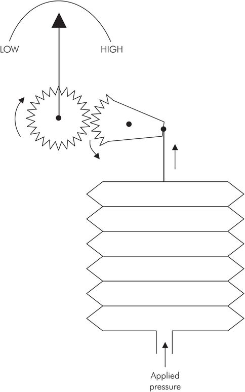
In the Bourdon gauge the measured pressure is connected to a spiral tube which uncoils as the pressure increases. This uncoiling movement is coupled to a pointer which indicates the pressure. Another form of aneroid mechanism relies on the expansion of a capsule produced by connection to the sampled pressure. This expansion again drives a pointer over a scale (Figure 45.15).
Advantages – simple technology, mechanically robust and convenient to use. Operate in any position and do not require power supply. Suitable for high or low pressures.
Disadvantages – not suitable for very low pressures (< 5 cmH2O). Not easily recalibrated.
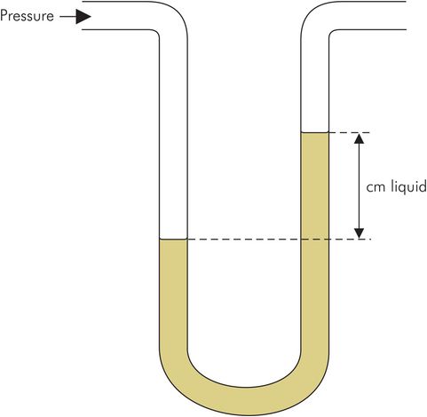
Manometer
This is the most basic device for measuring pressures, and because of its simplicity it represents a standard method of calibrating other devices. The unknown pressure is measured by balancing it against the pressure due to a column of a liquid (Figure 45.16). The liquids used most commonly are water for lower pressures and mercury for higher pressures. The manometer is so fundamental to pressure measurement that pressure units commonly employed are cmH2O and mmHg. Accuracy and sensitivity can be increased by angling the manometer tubing and using a liquid with a lower density than water (e.g. alcohol). Surface tension between the liquid and the manometer tubing can cause an error, which causes the water manometer to read too high and the mercury manometer to under-read.
Advantages – simplicity of mechanism and no need for calibration. A standard method used to calibrate other techniques of pressure measurement.
Disadvantages – bulkiness of the device and lack of a direct reading.
Manometer
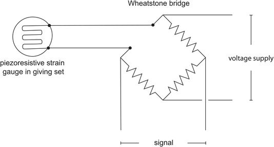
Piezoresistive strain gauge
This device is based on a semiconductor material with piezoresistive properties which cause it to vary in electrical resistance when subjected to a mechanical strain. The semiconductor is deposited onto the surface of a thin diaphragm which flexes when a pressure difference is applied across it. The distortion of the diaphragm produces a strain in the piezoresistive material which forms one arm of a bridge circuit (see Wheatstone bridge circuit in Chapter 44) etched onto the diaphragm. This results in a small signal current from the transducer which can then be amplified and processed (Figure 45.17).
Advantages – versatility, since it can be used for measurement of high or low pressures. The electronic signal and display make it suitable for online display, automated data logging and linking to a computer. It is also easily adaptable for measuring differential pressures, since the diaphragm can be mounted with each face of the diaphragm enclosed in its own chamber and isolated from the other. Differential pressures can be used to measure gas flows, with the use of a suitable pneumotachograph head.
Disadvantages – requires power supply and signal processing unit. Susceptible to electrical interference but has to be used in electronically hostile environments (operating theatres and intensive care units).
Blood pressure measurement
Blood pressure is an important determinant of tissue perfusion, oxygen delivery and cardiac work; it varies between individuals and is subject to a diurnal rhythm (lowest when the subject sleeps).
Recorded blood pressures reflect not only cardiovascular performance but also artefact (Figure 45.18).
| Cardiac output |
| The pulsatile nature of blood flow |
| Systemic vascular tone |
| Hydrostatic pressure variation in the circulatory system |
| The characteristics of the measurement system used |
Failure to recognise this can result in errors of interpretation and inappropriate action.
Variation due to the site of measurement
Changing the site of measurement, such as altering the level at which an arterial pressure transducer is positioned, will alter the blood pressure reading obtained because of the hydrostatic pressure difference between the transducer positions. For this reason, a standard reference point is taken, usually the level of the heart (right atrium), so that all pressures measured are relative to that in the right atrium.
Changing the measurement site by 10 cm in height produces an error of 7.5 mmHg in the blood pressure measurement.
Since blood flow is pulsatile, the blood pressure varies according to the phase of the cardiac cycle. Thus peak (systolic), trough (diastolic) and mean pressures are defined individually, when discussing blood pressure measurements.
Methods of measuring blood pressure
The value of the displayed blood pressure is a function of the method used to measure it. The validity of any such measurements is strongly influenced by the observer’s familiarity with the particular strengths/weaknesses of the technique employed. These can be divided into indirect and direct methods.
Indirect methods of measuring blood pressure
These methods are most commonly based on an occlusive cuff, which is inflated to a pressure above that of the artery and then slowly deflated. Once the cuff pressure falls below that of the artery peak pressures, pressure transients begin to pass beneath the cuff. These transients can be detected by a ‘sensing’ cuff, by manual palpation or by auscultation, and the pressure in the occluding cuff can then be recorded. In this way systolic and diastolic blood pressure values can be derived from these pressure transients, and can be measured manually or automatically.
Manual occlusive cuff methods
Manual methods rely on auscultation and palpation and are historically the earliest, but have become superseded by automated non-invasive techniques, which provide a continuous display of blood pressure. These manual methods, however, provide a historical perspective.
Riva-Rocci (1896) – described the use of an occlusive cuff to measure systolic pressure by palpation.
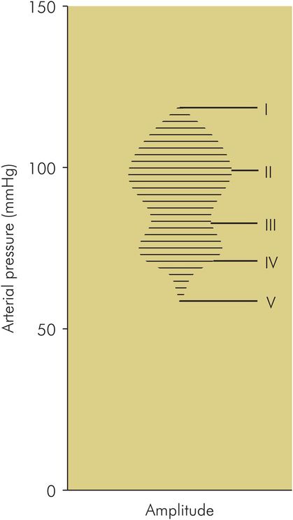
Korotkov (1905) – again using an occlusive cuff, Korotkov first described the measurement of blood pressure by auscultation. ‘Korotkov sounds’, heard over the artery as the cuff pressure falls, are the result of turbulent blood flow, vibration in the arterial wall, and pressure transients created as the extent of arterial occlusion decreases (Figure 45.19):
Phase I – a clear tapping synchronous with the pulse.
Phase II – sounds become softer approximately 5–10 mmHg below phase I.
Phase III – as the diastolic point approaches, sounds become more intense.
Phase IV – sounds suddenly become muffled, then, 5–10 mmHg later,
Phase V – sounds disappear.
Von Recklinhausen (1931) – described a dual cuff (occlusive and sensing) technique, employing aneroid valves in series within a sealed metal block, the oscillotonometer. This provided a visual measure of systolic, diastolic and mean arterial pressures displayed on a dial, connected by levers to an aneroid gauge.
Korotkov sounds
Flush method
This is an occlusive cuff method used for neonates. The arm is milked of blood before inflation of the occlusive cuff, which is then slowly deflated. The systolic point corresponds to the pressure at which flushing of the arm occurs (this point more closely reflects the mean arterial pressure).
Automated occlusive cuff methods (oscillometry)
Oscillometry is the most common method of automatic blood pressure measurement in clinical practice and is a development of Von Recklinhausen’s oscillotonometer. The accuracy of blood pressure measurement has been improved by coupling the rate of cuff deflation to heart rate. A single occlusive cuff is employed using a dual sensing connection, which replaces the double cuff of the oscillotonometer. A pneumatic pump periodically inflates the cuff to a point 25–30 mm Hg above the systolic pressure and allows air to escape through a bleed valve, producing controlled deflation (approximately 2–3 mmHg s–1). Vibrations of the arterial wall produce pressure transients which are transmitted via a sensing channel to an electrical transducer in the apparatus. The data is then analysed by a microprocessor which calculates systolic, diastolic and mean arterial pressures. The effects of electrical noise are reduced by comparing successive arterial pulsations as the cuff pressure decreases. If these do not correlate the data are rejected.
An example of pressure transients during cuff deflation is shown in Figure 45.19.
Systolic pressure corresponds to the point where the amplitude of pulsations is increasing, and is approximately 25–50% of maximum. Diastolic pressure corresponds to the point where the amplitude of pulsations has declined to 80% of the maximal pulse amplitude. Mean arterial pressure is the maximum amplitude point.
Advantages – the principal advantages of these instruments is that they free the operator’s hands, allowing measurements to be obtained conveniently when access to the patient is difficult, allow calculation of the mean arterial pressure, include alarm capabilities, and provide the capacity for data transfer.
Disadvantages – while correlating fairly well with invasive measurements, they are less accurate at extremes of blood pressure (will over-read at low pressures and under-read at high pressures), and should not be regarded as any more accurate than manual techniques. All these instruments assume the presence of a regular cardiac cycle; when this is absent, e.g. in atrial fibrillation, blood pressure measurements become inconsistent. The automatic cuff increases the risk of underlying tissue damage (in the elderly, particularly when the frequency of measurement is high, and the instrument is used for prolonged periods). Incorrect cuff placement may be responsible for nerve entrapment injuries (the ulnar nerve at the elbow).
Penaz technique
In oscillometry blood pressure measurement relies on gradual deflation of a cuff, which limits the frequency of measurement (maximum frequency of measurement is usually 1 min–1). To overcome this limitation, a continuous non-invasive technique was first described by Penaz in 1973. This monitors the diameter of the digital artery using an infrared plethysmograph, which is mounted in a pneumatic cuff. The infrared signal responds to arterial dilatation and contraction during each cardiac cycle. This infrared signal is used to servocontrol a pump which maintains it at a constant level corresponding to mean arterial pressure, by inflating and deflating the cuff. Thus as the artery dilates in systole cuff pressure is increased, and as arterial diameter reduces during diastole, cuff pressure decreases. This duplicates the arterial pressure wave form in the cuff, which is then displayed on the machine.
Advantages – this method provides a record of the changing trends in blood pressure, and in patients with normal or vasodilated fingers it correlates well with invasive methods.
Disadvantages – results are less reliable in patients with peripheral vascular disease. Small differences in cuff positioning/tightness result in significant changes in the measured pressure. These measurements display a downward drift because of relocation of tissue fluid, necessitating repeated calibration. When used for periods in excess of 20–30 minutes, the cuff causes discomfort; where there is poor peripheral blood flow, there is the potential for vascular occlusive damage.
Continuous arterial wall tonometry
An alternative to the Penaz technique monitors changes in arterial wall elasticity/tonometry. A standard arm cuff is inflated to a constant low pressure (usually 30 mmHg), and the instantaneous changes in cuff pressure that result from arterial distension are interpreted by complex algorithms. Evaluation of response and accuracy of this device is mixed; the general impression is that at best it provides only a fair comparison with direct methods.
Doppler ultrasound
This method employs a transducer probe which transmits and receives ultrasound waves. These are coupled to the skin by a layer of gel, and positioned directly over the artery. Movements in the arterial wall caused by pressure transients as they pass beneath the cuff cause Doppler shifts in the frequency of the transmitted ultrasound waves. The amplitude of the shift provides a measure of the systolic and diastolic pressures. This technique should not be confused with the Doppler detection of blood flow in arteries, which analyses the reflection of ultrasound from the red blood cells in the vessel.
Advantages – can be used for patients of all ages.
Disadvantages – requires the accurate positioning of the transducers, and the use of the correct ultrasound coupling medium. The signals are prone to movement artefact, and are distorted by diathermy, dysrhythmias and atrial fibrillation.
Sources of error in indirect methods
In comparison with direct methods of blood pressure measurement (taken as the gold standard), indirect methods tend to slightly under-read, with the diastolic pressure showing the greatest degree of variability. The sources of error include:
Korotkov sounds – these are complex sounds, with a large proportion of the sound energy being below the audible range. This reduces sound transmission to the observer. In addition, observer detection of the sounds will be dependent on aural acuity. The generated sounds are flow-dependent, and thus factors affecting flow can introduce inaccuracy (e.g. in high-output states, and after exercise, phase V may not occur)
Cuff size – the width of the cuff affects the measured value of blood pressure. When too narrow, there is a tendency to overestimate; if too wide, underestimation occurs. As a consequence, there have been efforts to standardise the widths of blood pressure cuffs. The World Health Organization (WHO) recommends that adult cuffs should be 14 cm wide, and should cover two-thirds of the length of the upper arm, or its width should be 20% greater than the diameter of the arm. Suggested widths are shown in Figure 45.20.
Zero/calibration errors – particularly in aneroid devices.
Pneumatic leaks – recommended working life for cuffs
Speed of deflation – when too fast, then there is insufficient time to detect audible change.
Direct method: intra-arterial pressure monitoring
This provides an invasive, continuous measure of blood pressure by beat-to-beat reproduction of the arterial pressure waveform. It is particularly useful:
In patients with cardiovascular instability
Where blood pressure manipulation is required (inotropes or vasodilators)
Where non-invasive blood pressure measurement is likely to be difficult and/or inaccurate (obesity)
The method requires the insertion of a short parallel-sided cannula into an artery. A continuous flow of either saline or heparinised saline (1 U mL–1) at rates between 1 and 4 mL h–1 is used to reduce clot formation in the cannula. The cannula is connected by a short length of narrow-bore non-compliant plastic tubing containing saline to a pressure transducer, which is usually of the piezoresistive strain gauge type. More recently catheter tip pressure transducers have been developed but remain comparatively expensive. As noted above, the piezoresistive strain gauge produces a low-amplitude signal requiring signal processing before analysis and display.
The design of an intraarterial pressure monitoring system must take into account the following considerations:
The frequency and phase shift responses of the system have to be adequate to allow good reproduction of the arterial signal. An approximate guide is that acceptable accuracy requires a frequency response extending to 8–10 times the maximum heart rate expected. In humans, the most important information is contained within the frequency range 0–20 Hz. The system can thus be designed to have an upper cutoff frequency > 20 Hz.
The transducer and connecting tubing should be chosen to avoid natural frequencies or resonances occurring within the desired frequency response. Mechanical resonances due to the properties (compliances and inertial elements) of the transducer and column of saline in the connecting tubing can be shifted above the desired cutoff frequency by reducing the diameter of the connecting tubing.
Components must also be chosen to provide the optimum degree of damping. Usually ‘critical damping’ is aimed for, but since frequency response, phase shift response and damping requirements may conflict a compromise may have to be arrived at. It is important to be able to recognise abnormal levels of damping in order to interpret the arterial waveforms appropriately. Figure 45.21 illustrates over-damping, under-damping and appropriate damping of arterial waveforms.
Advantages – this method provides a continuous display of the pressure wave form, providing an immediate assessment of blood pressure which is regarded as the gold standard.
Disadvantages – as with any invasive technique, there are potential problems:
Cannulation – this can be difficult, particularly in low-output states, and may require consideration of multiple sites before success.
Disconnection – if unrecognised, this may result in serious blood loss and, in the extreme, exsanguination.
Infection is particularly relevant in cases of prolonged use (e.g. in the intensive care unit). Aseptic technique at the time of insertion, care of the catheter site (including appropriate dressing), and use of sterile packaged single-use manometer sets is necessary.
Vascular damage – distal vascular insufficiency may result directly from cannulation, or arise from subsequent thrombosis of the cannulated artery. This risk is increased by insufficient collateral circulation, which should always be checked for before cannulation. Emboli (air or thrombus) can cause distal vascular occlusion.
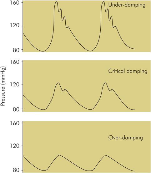
Effect of measurement system damping on the arterial pressure waveform
Sources of error in arterial pressure monitoring
Air bubbles – as noted above, a recording system with a high resonant frequency and critical damping is preferable. Standard pressure transducers have a natural frequency in the region of 100 Hz, but the addition of the connecting tubing, tap and cannula markedly reduces this. The presence of air bubbles in the system also decreases the resonant frequency of the system and increases the damping.
Catheter wall compliance – if compliant tubing is used to connect the cannula and transducer it will distend with the pulse wave, and like the presence of air will cause decreased resonant frequency and increased damping.
Blood clot – if this forms within the cannula it will increase the flow resistance of the cannula and also the flow velocity of the saline. These factors will also tend to increase system damping and decrease resonant frequency.
Zero point – the importance of choosing a zero reference point in order to minimise hydrostatic errors has been described above. This effect can be reduced by periodic zeroing of the system.
Gas flow measurement
The measurement of gas flow and volumes is applied in clinical practice for the following applications:
To test pulmonary function in patients
To monitor gas flows in anaesthetic machines
To monitor respiratory flows and tidal volumes in patient breathing circuits
Devices used in pulmonary function testing are described below.
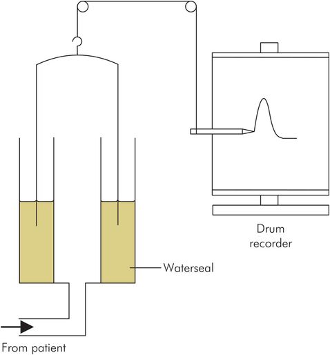
Benedict Roth spirometer
This consists of a light bell which traps a closed volume of air over water. The subject breathes in and out of this trapped gas, causing the bell to rise and fall following the inspired and expired volumes. A sensor or pen coupled to the bell traces its movement, giving a spirometric trace from which gas flow rates and lung volumes can be derived (Figure 45.22). This device is relatively large in size and not portable.
Benedict Roth spirometer
Vitalograph
The vitalograph records expiratory flow rates and volumes by collecting expired gas from the subject in a bellows. A recording pen is coupled to the bellows, tracing an expired volume graph (Figure 45.23). This device is more portable than the Benedict Roth spirometer but only measures forced expiratory volumes and flows. The results obtained are also very dependent on subject technique.
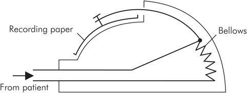
Vitalograph
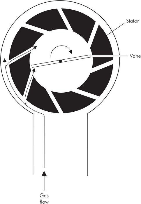
Wright respirometer
This is another continuous volume recorder, designed specifically for clinical application. It operates by using the gas flow to drive a spinning vane, which is coupled by clockwork gears to the display dials. Total volumes up to 1000 litres can be recorded. Like the dry gas meter, its accuracy and reliability is dependent on the mechanical quality of its clockwork mechanism. It can only measure unidirectional flow but has the advantages of being small and portable, and requiring no power supply. Flow rates again can only be derived by averaging recorded volumes over time (Figure 45.24).
Dry gas meter
This machine is based on the gas meters used for measuring domestic gas consumption. It measures large volumes of gas by continually feeding the gas flow into a pair of reciprocating bellows. As each bellows fills alternately, its movement records an increase in volume by a clockwork counter and operates inlet and exhaust valves to direct the gas flow through the machine. In this way the flow of very large volumes (106 litres) of gas can be measured, compared to the several litres capacity of the closed-volume spirometers. However, average flow rates can only be estimated over time, and cannot be measured directly.
Electronic volume meter
In this device the spinning vane mechanism described above in the Wright respirometer has been adapted to give an electronic signal. One method uses fixed blades to create a spiral flow to drive the blades of the vane. The spinning blades interrupt a light signal from light-emitting diodes (LEDs), which is then picked up by photoelectric cells. These provide an electrical signal which can be processed and calibrated to give volume measurements. This device has the advantages of being free from the mechanical errors associated with clockwork mechanisms, and being able to measure volumes from bidirectional (inspiratory and expiratory) flow. It does, however, require a power supply, and a signal processing and display unit.
Peak flow meter
This device records the maximum expiratory flow of patients by using the expired gas to operate a shutter controlling a variable orifice through which the gas escapes to the atmosphere. The greater the expiratory flow, the larger the orifice opened up by the shutter. The displacement of the shutter is non-returnable and is recorded by a pointer which thus records the maximum expiratory flow reached (Figure 45.25).
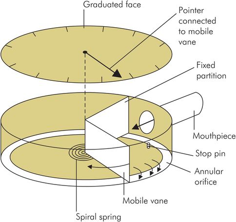
Peak flow meter
Gas flow measurement in anaesthetic machines
Rotameter
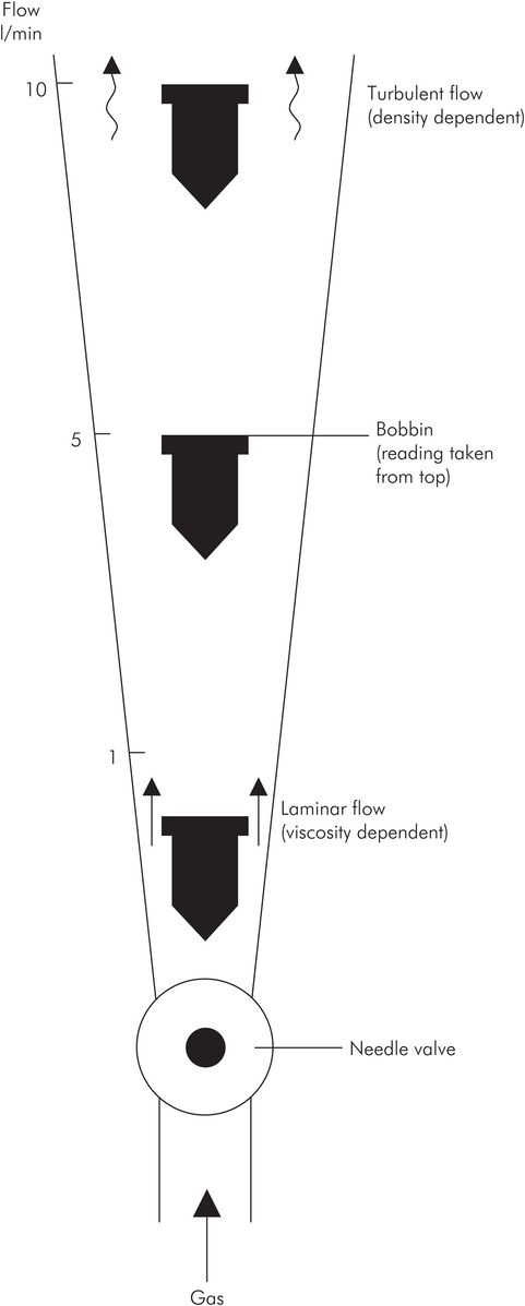
Gas flows from an anaesthetic machine into a ventilator or patient circuit are most commonly measured using rotameters. The rotameter is a variable-orifice flow meter in which the gas flow to be measured is passed upwards through a vertically mounted glass (or plastic) tube. This tube has a tapering internal diameter, wider at the top and narrower at the bottom. Gas flow through the rotameter is controlled by a needle valve at the bottom (Figure 45.26).
Rotameter
A bobbin with a smaller diameter than the internal diameter of the rotameter tube acts as a pointer, and is moved up or down the tube by the force of the gas flow as it increases or decreases. The bobbin may vary in design, but the most common type is shaped like a spinning top, with spiral grooves cut in the sides causing it to spin in the gas flow. The spin reduces friction and sticking of the bobbin. With this type of bobbin, readings are taken from the top edge.
When the gas flow is steady the bobbin settles at a point where the force of the gas flow acting on it and passing round it equals the bobbin weight. At high flows the bobbin is near the top of the rotameter and the cross-section of the annular space around the bobbin is greater than at low flows, when the bobbin is near the bottom of the rotameter and the orifice cross-section is small.
Gas flow pattern in a rotameter
The pattern of gas flow through a rotameter is a mixture of turbulence and laminar flow, due to the flow conditions as the gas passes the bobbin. When the cross-sectional area open to flow is small (i.e. the bobbin is near the bottom of the rotameter), flow past the bobbin is like flow in a ‘tube’. This is because the cross-sectional area open to flow is small, and a tube in this context is defined by having diameter < length (see Flow through tubes in Chapter 44). In this case flow is laminar and gas viscosity is the main determinant of flow. When the bobbin is near the top of the rotameter, at high flows, the annular cross-sectional area open to flow is large. Flow here is similar to that through an ‘orifice’, an orifice being defined by having diameter > length. In this case flow is turbulent and density becomes the most important gas property determining flow. The importance of the flow pattern is that because the viscosities and densities of gases can differ significantly (e.g. oxygen and helium have similar viscosities but their densities are 1.33 and 0.17 kg m–3), a rotameter can only be calibrated accurately for a specific gas or mixture.
Advantages – simple design and reliable, does not require power supply, no signal transmission path, conditioning unit or display to go wrong.
Disadvantages – only calibrated for specific gas under standard pressure and temperature conditions. Actually part of the gas circuit, so failure may be hazardous, and sensitive to circuit changes downstream (see below).
Related posts:


Stay updated, free articles. Join our Telegram channel

Full access? Get Clinical Tree


