which is graphically demonstrated in Figures 26.4, 26.5 and 26.6.
In this chapter the steps in the derivation of this and other equations are shown in boxes.
In this chapter the term ‘drug’ is used for molecules binding to receptors, although the model applies equally to other molecules (ligands) that bind to receptors.
- Initial terms used
- ⇒
- ⇒
implies that
- ∝
proportional to
- Square brackets [ ]
are used to indicate a concentration
- [D]
concentration of free drug
- [R]
concentration of unoccupied receptors
- [DR]
concentration of drug-occupied receptors
- k1
constant that defines the rate of the association (forward) reaction
- k2
constant that defines the rate of the dissociation (backward) reaction
- KD
constant (the dissociation constant) that defines the equilibrium point of the whole interaction
Concentration–effect relationships
Drug–receptor kinetics
The essential pharmacodynamic interaction is that of a drug binding reversibly to a receptor to form a drug–receptor complex.
We will use the interaction of noradrenaline (norepinephrine) with an α1-adrenoceptor to illustrate the concept (see Chapter 28 for details on receptor binding sites).
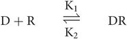
The law of mass action states that the velocity of a chemical interaction is proportional to the molecular concentrations of the reacting components.
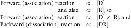
For clarity the multiplication sign is usually omitted, and [D] × [R] is written as [D][R].
The next step is to insert the constants to convert ∝ to =, which results in the two terms:
At equilibrium, there is no net change in the balance of concentrations and the rate of association reaction equals the rate of the dissociation reaction, so k1[D][R] = k2[DR]
This can be rearranged as:

In any equation, constants can be combined as a single constant. In this case, the ratio of the two constants k1 and k2 is called the equilibrium or dissociation constant, which is termed KD.
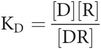
The final step is to substitute one constant for two, which leads to Key equation 1:
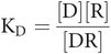
Key equation 1
Key points
KD is called the dissociation (or equilibrium) constant.
KD is a constant for a particular drug–receptor interaction and defines that interaction.
KD permits quantitative comparisons of the equilibrium points of different drug–receptor combinations (e.g. noradrenaline with α1-receptor, noradrenaline with α2-receptor and adrenaline with α1-receptor all have different values for KD).
The reciprocal of the dissociation constant is called the affinity of the drug for the receptor. In other words:
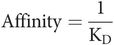
The higher the affinity of the receptor for the drug then the more associated (less dissociated) it is, so the lower the dissociation constant and vice versa.
Example
An example KD for noradrenaline and the α1-adrenoceptor is 10–7 molar (100 nanomoles L–1).
While the dissociation constant is very important, the equation itself is of limited use. What is required is the relationship of occupancy (the proportion of receptors occupied by the drug) to drug concentration.
Additional terms used
- r
receptor occupancy
- RT
total number of receptors
So, occupancy 
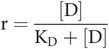
Key equation 2
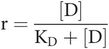
This equation relates occupancy to drug concentration and the dissociation constant for the drug–receptor combination.
To derive Key equation 2 the receptor term [R], not featuring in occupancy (r), must be substituted in Key equation 1.
The total number of receptors is the sum of free and drug-bound receptors
Substituting [R] from Key equation 1 gives
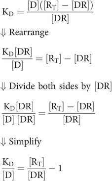
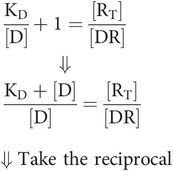
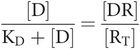
Substitute the term for occupancy (r)
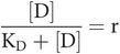
This is Key equation 2:
Key points
When the drug concentration is zero, occupancy will be zero.
When the drug concentration is equal to KD then occupancy will be ½.
As drug concentration rises the dissociation constant becomes very small in relation to the concentration, so occupancy will reach close to 100%.
These features will become apparent in the charts later in the chapter.
In our example using noradrenaline, at a noradrenaline concentration of 100 nmol L–1 at any particular time at equilibrium, half of the α1-receptors will be occupied as a drug–receptor complex.
In the model, the occupancy relationship is important for explaining how pure agonists behave, but it also applies equally to partial agonists, competitive antagonists and inverse agonists.
To make full use of the model, a term to describe the effect that is produced is required.
Additional terms used
- R
response (not the same as [R] in earlier equations)
- E
efficacy (a constant for a drug–receptor complex)
The receptor response produced by an agonist binding with the receptor is a function of the occupancy and the effect (efficacy) of the agonist on that receptor. For the purpose of this model, response (R) is proportional both to occupancy (r) and to the efficacy (E) of the drug–receptor complex:
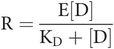
Key equation 3
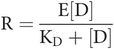
Key points
When the drug concentration is zero, response will be zero.
When the drug concentration is equal to KD then response will be ½ that of the efficacy.
As drug concentration rises the dissociation constant becomes very small in relation to the concentration, so response will reach close to 100% of maximum.
These features will also become apparent in the charts later in the chapter.
In our example using noradrenaline, at equilibrium at a noradrenaline concentration of 100 nmol L–1 the response from the α1-receptors will be half of the maximal response.
Efficacy and drug–receptor interactions
Graphical plots based on Key equation 3 are used to demonstrate and explain the features of the drug–receptor interactions. These are classified in Figure 26.2. Non-competitive and non-reversible antagonists produce no response. The plots are purely a graphical demonstration of Key equation 2 or Key equation 3 above.
| Type of drug–receptor interaction | Efficacy | Response maximum from that drug |
|---|---|---|
| Pure agonist | 1 | Full |
| Partial agonist | Between 0 and 1 | Some response but never maximal |
| Reversible competitive antagonist | 0 | No response |
| Inverse agonist | Negative value | Opposite effect |
In this section A and B are introduced to represent different pairs of drugs, and so the following additional terms are used:
- [B]
concentration of antagonist
- [BR]
concentration of receptors occupied by the antagonist
- [DA]
concentration of agonist
- [DB]
concentration of antagonist
- rA
occupancy of receptor by agonist
- rB
occupancy of receptor by antagonist
- KA
equilibrium constant for defining the agonist–receptor interaction (replaces KD from previous section)
- KB
equilibrium constant for defining the antagonist–receptor interaction
Do not confuse the terms KA and KB with the terms Ka and Kb used in acid–base calculations.
Figure 26.3 lists the values used in the graphical examples that follow. Note that the values for equilibrium constants are not actual ones but represent concentrations for the purposes of illustration.
| Ligand | Abbreviation | Dissociation constant | Efficacy |
|---|---|---|---|
| Agonist 1 | A1 | 50 | 1 |
| Agonist 2 | A2 | 25 | 1 |
| Agonist 3 | A3 | 100 | 1 |
| Partial agonist 1 | P1 | 50 | 0.75 |
| Partial agonist 2 | P2 | 500 | 0.75 |
| Reversible competitive antagonist | B | 450 | 0 |
| Irreversible competitive antagonist | I | 0 |
Related posts:



Stay updated, free articles. Join our Telegram channel

Full access? Get Clinical Tree