Cardiac muscle structure
A further difference from skeletal muscle lies in the electrical conductive characteristics of the cardiac muscle fibres, which offer a low resistance to the propagation of action potentials along the axis of muscle cells, owing to the intercalated discs. The intercalated discs allow rapid transmission of action potentials between cells via gap junctions which are composed of connexons or open channels connecting the cytosol of adjacent cells.
Finally, cardiac muscle cells contain much greater numbers of packed mitochondria and are more richly supplied with capillaries than skeletal muscle, since the myocardium cannot afford to incur an oxygen debt by using anaerobic metabolism.
The actin–myosin coupling and decoupling reaction lies at the heart of the contractile process and is fuelled by ATP and calcium.
The sarcoplasmic reticulum acts as a reversible intracellular store for calcium ions.
Cardiac muscle is a functional syncytium with an all-or-nothing contractile response
Excitation–contraction coupling
This term describes the events which are initially triggered by an action potential and which culminate in contraction of a myofibril. Propagation of an action potential along the sarcolemma and into the muscle cell through the T-tubule system causes calcium ions (Ca2+) to enter the cell through voltage-dependent and receptor-dependent channels, and also by passive diffusion across the sarcolemma. This initial rise in Ca2+ triggers further release of Ca2+ from the sarcoplasmic reticulum. As a result intracellular Ca2+ levels increase from resting values of 10−7 mmol L−1 to concentrations of 10−4 mmol L−1 (Figure 14.2). The released calcium acts on the thin filaments, binding to troponin C and causing tropomyosin to move and reveal the actin binding sites for the myosin heads. This enables the myosin heads to attach themselves to the actin filaments, and contraction commences. Contraction proceeds by a ‘walk-along’ or ‘ratchet’ process, in which ATP is hydrolysed to ADP by ATPase in the myosin head. The energy released produces the ‘power stroke’ that slides the myosin on the actin.
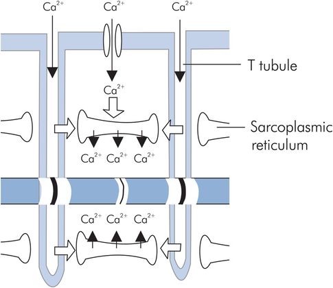
T tubule and sarcoplasmic reticulum structure
The strength of cardiac muscle contraction is highly dependent on the calcium concentration in the extracellular fluid. At the end of the action potential plateau the calcium flow into the cell decreases, and the intracellular Ca2+ is actively pumped back into the sarcoplasmic reticulum and T tubules by a calcium–magnesium ATPase pump. The chemical interaction between actin and myosin ceases and the muscle relaxes until the next action potential.
Cardiac action potentials
An action potential (AP) is a spontaneous depolarisation of an excitable cell’s membrane, usually in response to a stimulus.
Two different types of action potential are found in the heart, the fast-response and the slow-response. In the myocardium two cell types produce fast-response action potentials. These are the contractile myocardial cells and the conduction system cells. Slow-response APs are normally produced by the pacemaker cells in the sinoatrial (SA) node and the atrioventricular (AV) node. These pacemaker cells spontaneously depolarise to produce slow-response APs, exhibiting a property called automaticity.
Fast-response action potential
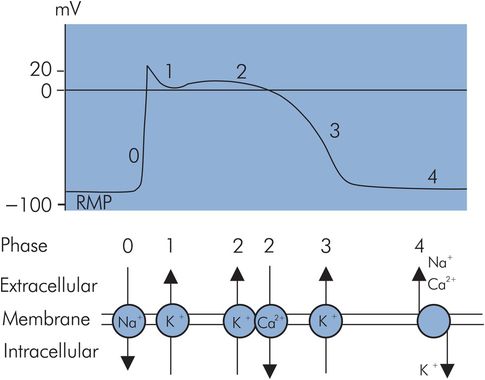
The fast-response AP of the cardiac muscle cell can be divided into five distinct phases (Figure 14.3):
Phase 0 – initial rapid depolarisation/upstroke
Phase 1 – early rapid repolarisation
Phase 2 – prolonged plateau phase
Phase 3 – final rapid repolarisation
Phase 4 – resting membrane potential
Fast-response action potential
Resting membrane potential (RMP)
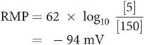
The RMP is the electrical potential across the cell membrane during diastole and is approximately –90 mV, the intracellular membrane surface being negative with respect to the extracellular surface. The RMP is maintained by the permeability properties of the cell membrane, which retains negative ions (anions) in the cell but allows positive ions (cations) to diffuse out of the cell. The cell membrane is impermeable to negatively charged ions such as proteins, sulphates and phosphates, which therefore remain intracellular. In contrast membrane permeability to potassium is higher, allowing it to diffuse out of the cell under its concentration gradient of approximately 30:1. Potassium diffuses out of the cell until an equilibrium is reached at which the electrostatic attraction of the retained anions balances the chemical force moving the potassium down its concentration gradient out of the cell. This equilibrium is expressed mathematically by the Nernst equation.
The intracellular–extracellular concentration gradient of potassium must be maintained if the RMP is to stay constant. This is achieved by the active transport of potassium from the extracellular fluid to the intracellular space by a sodium–potassium pump.
Other ions also contribute to the RMP by producing transmembranous potentials due to the balance between chemical and electrostatic forces acting on them. For instance, sodium will diffuse across the cell membrane in the opposite direction to potassium (i.e. extracellular to intracellular) because of the normal resting sodium concentration gradient. Accordingly this movement of sodium into the cell will reduce the membrane potential set up by potassium. However, because membrane permeability to sodium under resting conditions is relatively low, this effect is small, only reducing the membrane potential by approximately 4 mV. Similarly the cell membrane is relatively impermeable to other ions in the resting state, and therefore the RMP is primarily determined by the intracellular/extracellular distribution of potassium ions.
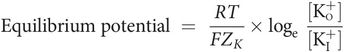
where
[K+I] = potassium concentration inside cell membrane
[K+o] = potassium concentration outside cell membrane
R = the gas constant
T = absolute temperature
F = Faraday’s constant
ZK = the valency of potassium
Thus:
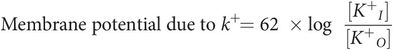
But resting membrane potential (RMP) is due mainly to the distribution and diffusion of potassium ions (see below), therefore:
Phase 0 – rapid depolarisation
An action potential is produced when an electrical stimulus increases the RMP (causes it to become less negative) to a threshold potential (TP). At this value, fast sodium channels open for a very short period of time and potassium channels close. Sodium rapidly enters the cell under the influence of its concentration gradient and the electrostatic attraction of the intracellular anions, to make the inside positive in comparison to the outside by +20 mV. At the end of this stage the sodium channels close. This phase coincides with the ‘all-or-nothing’ depolarisation of the myocardium and the QRS complex of the ECG.
The retention of many intracellular anions (proteins, phosphates and sulphates) to which the cell membrane is not permeable.
The selective permeability of the cell membrane, which is almost 100 times more permeable to potassium than to sodium, allowing potassium to flow down its concentration gradient out of the cell while keeping sodium extracellular.
The maintenance of an intracellular–extracellular concentration gradient for potassium ions by a sodium–potassium ATPase pump. This transports potassium actively into the cell and sodium out of the cell (three Na+ ions for every two K+ ions) and is dependent on energy supplied by the hydrolysis of ATP.
Phase 1 – early rapid repolarisation
This describes a brief fall in membrane potential towards zero following the rapid rise in phase 0. This occurs due to the start of potassium flow out of the cell under the positive intracellular electrical gradient and chemical gradients. At the same time slow, L-type Ca2+ channels open, providing a prolonged influx of calcium ions which maintains the positive intracellular charge. There is also movement intracellularly of chloride following sodium into the cell along the electrical gradient. All of this leads to an initial rapid repolarisation of the cell membrane to just above 0 mV.
Phase 2 – plateau phase
During this phase the continued influx of calcium via the slow L-type Ca2+ channels is balanced by the continued efflux of potassium commenced in phase 1. This maintains the zero or slightly positive membrane potential and corresponds in time with the ST segment of the ECG.
Phase 3 – final rapid repolarisation
Potassium permeability rapidly increases at this stage and potassium flows out to restore the transmembrane potential to –90 mV. Although repolarisation of the membrane is complete by the end of phase 3, the normal ionic gradients have not yet been re-established across the membrane
Phase 4 – restoration of ionic concentrations and resting state
During this phase ATPase-dependent ion pumps exchange intracellular sodium and calcium ions for extracellular potassium, thus restoring the resting ionic gradients. When an equilibrium state is reached electrostatic forces equal the chemical forces acting on the different ions and RMP is re-established. This phase corresponds to diastole.
Atrial cell action potentials
Atrial myocyte action potentials are also of the rapid-response type but vary from the ventricular action potentials in having a shorter-duration plateau (phase 2). This effect is due to a much greater early repolarisation current (phase 1) in the atrial AP than in the ventricular case (Figure 14.4).
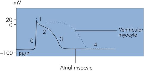
Atrial and ventricular myocyte action potentials
Excitability of cardiac cells
Excitability describes the ability of cardiac tissue to depolarise to a given electrical stimulus. It is dependent on the difference between RMP and TP, and thus changes in RMP will alter myocardial excitability. When RMP decreases (becomes more negative), this difference becomes greater and the heart becomes less excitable. Similarly, excitability is increased as the difference between RMP and TP decreases. Various factors affect excitability, including:
Catecholamines
β-Blockers
Local anaesthetics
Plasma electrolyte levels
Refractoriness
During rapid depolarisation (phase 0) and the early part of repolarisation (phases 1, 2 and the initial part of 3), the cell cannot be depolarised to produce another AP regardless of stimulus strength. The sodium and calcium channels are inactivated and repolarisation must occur before they can open again. This is called the absolute refractory period. During the latter part of phase 3 and early phase 4 a stronger than normal impulse can lead to an AP. This is called the relative refractory period. During this period the heart is particularly vulnerable because an impulse at this time might produce repetitive, dyssynchronous depolarisation (e.g. ventricular fibrillation or tachycardia). The absolute and relative refractory periods together form the effective refractory period.
Pacemaker cells
The heart continues to beat even after all nerves to it are sectioned. This happens because of the specialised pacemaker tissue (P-cell) that makes up the conduction system of the heart. These cells are found in the SA and AV nodes and also in the His–Purkinje system. Pacemaker cells exhibit automaticity (the ability to depolarise spontaneously) and rhythmicity (the ability to maintain a regular discharge rate). Normally atrial and ventricular myocardial cells do not have pacemaker ability, and they only discharge spontaneously when injured. There are however latent pacemakers in other parts of the conduction system that can take over when conduction from the SA and AV nodes is blocked.
Slow-response action potential
The action potential produced when a pacemaker cell depolarises spontaneously is called a slow-response action potential (Figure 14.5). The most negative potential reached just before depolarisation is called the maximum diastolic potential (MDP), which is only –60 mV compared to the RMP of –90 mV for a myocardial muscle cell. The reason for this is that the pacemaker cell membranes are more permeable to sodium ions in their resting state. Phases can be identified in the slow-response action potential which correspond superficially to some phases of the rapid-response AP, although the underlying events differ.
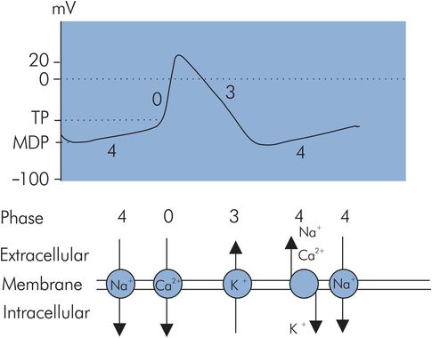
Slow-response action potential
Phase 4 – restoration of ionic gradients and resting state
These cells do not maintain a stable RMP, but instead depolarise spontaneously because of increased membrane permeability to cations during this phase. Sodium and calcium slowly ‘leak’ into the cell. Although potassium diffuses out simultaneously during this phase, the inward ‘leak’ of sodium predominates to cause the membrane potential to gradually increase until a threshold potential (TP) is reached at approximately –40 mV. This property is called spontaneous diastolic depolarisation or pacemaker automaticity, and is directly related to the positive slope of phase 4.
Phase 0 – rapid depolarisation
Rapid depolarisation occurs at TP and is mainly due to calcium influx through transient or T-type Ca2+ channels, which are slower than the rapid sodium channels responsible for phase 0 in the myocardial cell APs. The slope of phase 0 is therefore less steep than in the rapid AP case. The phase 0 slope in these cells is also reduced because of onset at a less negative transmembrane potential.
Phase 3 – repolarisation
In the slow response, repolarisation is effectively a single phase equivalent to phase 3 in the rapid response. Effectively phase 1 is absent and phase 2 is very brief, resulting in the absence of a plateau effect.
Pacemaker action potentials have the following features which differ from those of the myocardial cells:
Less negative phase 4 membrane potential
Less negative threshold potential
Spontaneous depolarisation in phase 4
Less steep slope in phase 0 (dependence on T-type Ca2+ channels)
Absence of phase 2 (plateau)
Ion channels and action potentials
Action potentials owe their basic characteristics to voltage-controlled changes in membrane permeability to different ions. The main ions concerned are potassium, sodium and calcium, whose membrane permeabilities are dependent on various types of ion diffusion channel. The basic ion diffusion channel is described in Chapter 10. These ion channels have been described in vitro by controlling and varying membrane potentials in different ion solutions, using a technique called ‘patch clamping’. Different channels can then be identified by the changes in current produced as the channels open and close according to their control potentials. Some of these channels are outlined in Figure 14.6.
| Action potential | Phase | Ion | Channel/gating mechanism |
|---|---|---|---|
| Rapid response (ventricular) | 0 | Na+ | Fast channels with ‘m’ activation and ‘h’ inactivation gates |
| 1,2,3 | K+ | Transient outward current (ito) channel | |
| 2,3,4 | K+ | Inward rectifier K+ current (iK1) channel | |
| 2,3,4 | K+ | Delayed rectifier K+ current (iK) channel | |
| 2 | Ca2+ | Slow (long-lasting, L-type) Ca2+ channel blocked by calcium antagonists | |
| Slow response (pacemaker) | 0 | Ca2+ | Transient (T-type) Ca2+ channel |
| 4 | Na+ | Specific channels ‘leaking’ sodium current (If) into pacemaker cells |
Automaticity of pacemaker cells
Automaticity is the ability of pacemaker cells to maintain a spontaneous rhythm, and it depends mainly on the leakage of sodium into the cell in phase 4 of the AP. This occurs via specific sodium channels which are activated when the membrane potential has become hyperpolarised, i.e. reached a value of approximately –50 mV during repolarisation. These channels then allow an inward hyperpolarisation current (If), which commences the spontaneous depolarisation of phase 4. The sodium current (If) is aided to a small extent by overlap of the decaying rapid depolarisation calcium current and opposed by extracellular diffusion of potassium. Automaticity is dependent on the slope of phase 4 of the AP, which is influenced by the autonomic system and various drugs.
Pacemaker discharge rate
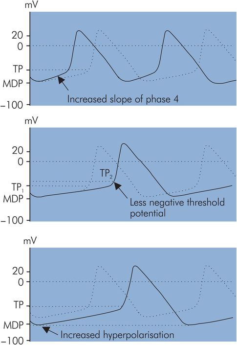
Pacemaker discharge rate is controlled primarily by the autonomic system. This is discussed in further detail later (see Heart rate, below). This control is mediated by changes in action potential characteristics. The following characteristics are associated with variation of the discharge rate (Figure 14.7):
Slope of phase 4 in AP – An increase in the slope of phase 4 reduces the time to reach TP during spontaneous depolarisation and thus increases pacemaker rate. Similarly a decrease in the phase 4 slope results in a slower pacemaker rate. Phase 4 slope can be varied by the autonomic nervous system.
Threshold potential – If this becomes less negative the pacemaker rate will decrease. Drugs such as quinidine and procainamide have this effect.
Hyperpolarisation potential – If hyperpolarisation is increased, i.e. the membrane potential becomes more negative, spontaneous discharge will take longer to reach TP during phase 4 and the pacemaker rate will decrease. This occurs with increases in acetylcholine levels.
Conduction system anatomy
The conduction system of the heart is composed of specialised cardiac tissues which form the following structures (Figure 14.8):
Sinoatrial node
Atrial conduction pathways
Atrioventricular node
Bundle of His
Bundle branches
Purkinje fibres
The sinoatrial (SA) node is the normal cardiac pacemaker, with a resting rate of between 60 and 100 per minute. It is a group of modified myocardial cells located close to the junction of the superior vena cava with the right atrium. Its blood supply is usually from a branch of the right coronary artery. Depolarisation spreads from the SA node through the atria and converges on the AV node.
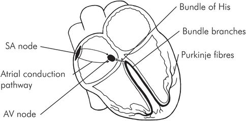
Anatomy of the conduction system
The two atria are electrically separated from the two ventricles except for three internodal communication pathways. The anterior (Bachmann), middle (Wenckebach) and posterior (Thorel) bundles connect the SA node to the AV node, which is located in the right posterior part of the right atrium close to the tricuspid valve and the coronary sinus opening. Anomalous accessory pathways (like the bundle of Kent) can sometimes connect the atria directly to the ventricle or other areas of the conducting system and cause a pre-excitation syndrome with arrhythmias. Blood supply to the AV node is also from a branch off the right coronary artery. The AV node is connected to the bundle of His, which distributes the impulse to the ventricles via the left and right bundle branches in the interventricular septum. There is a slight delay (about 0.13 seconds) of the impulse before it enters the AV node, inside the AV node and in the bundle of His. This delay permits completion of both atrial electrical activation and conduction before ventricular activation is started. The left bundle branch divides into the anterior and posterior fascicles. These bundles and fascicles run subendocardially down the septum and into the Purkinje system, which spreads the impulse to all parts of the ventricular muscle. Conduction velocity through the bundle branches and the Purkinje system is the most rapid of the conduction system. The AP as well as contraction begins endocardially and spreads out to the outside of the heart. However, repolarisation occurs from the outside to the inside. Ventricular activation is earliest at the apex and latest at the base of the heart, giving it an apical-to-basal contraction pattern.
Conduction system defects
Defects can arise in any part of the conduction system. Some examples of arrhythmias occurring due to lesions in different parts of the conduction system are shown in Figure 14.9.
| Site | Arrhythmia | Features |
|---|---|---|
| Sinoatrial node | Sick sinus syndrome | Sinus arrest, sinus bradycardia, tachycardias |
| Atrial conduction pathways | Wolff–Parkinson–White syndrome | Supraventricular tachycardia |
| Atrioventricular node | AV junctional rhythm | Bradycardia with abnormal P waves |
| Bundle of His | Complete (third-degree) AV block | Bradycardia with dissociated P waves |
| Bundle branches | Bundle branch block | Abnormal broad QRS complexes (> 0.12 s) |
The electrocardiogram
In an electrophysiological sense the heart consists of two chambers. The two atria function as a single electrophysiological unit and are separated from the biventricular unit by the fibrous atrioventricular ring. Electrical communication between these two units is only possible through the specialised conduction system. The main electrical events of the cardiac cycle are the mass depolarisation and repolarisation of the atria and ventricles. These can be thought of as waves of depolarisation (or repolarisation) which propagate through the cardiac tissues. As they propagate they generate potentials which can be sensed by electrodes on the skin surface. The electrocardiogram (ECG) is a recording of the signals picked up by a standard pattern of skin electrodes over the chest. When an electrode detects depolarisation moving towards it a positive deflection on the ECG is produced. Alternatively, if depolarisation is moving away from the electrode, it produces a negative deflection.
ECG waves and the cardiac cycle
The normal ECG consists of P, QRS, T and U deflections (Figure 14.10). Electrical activity precedes corresponding mechanical events during the cardiac cycle as follows:
The P wave is associated with atrial depolarisation and contraction. The atria repolarise at the same time as ventricular depolarisation, so the atrial repolarisation wave is usually obscured by the prominent QRS complex.
The PR interval is between the beginning of the P wave and the start of the QRS complex. This represents the time from onset of atrial contraction to the beginning of ventricular contraction. The normal PR interval is approximately 0.16 seconds, but it varies with heart rate.
The QRS complex reflects ventricular depolarisation and precedes ventricular contraction. A normal QRS complex has smooth peaks with no notches or slurs and has a duration of less than 0.12 seconds. The amplitude is dependent on multiple factors including myocardial mass, the cardiac axis, the distance of the sensing electrode from the ventricles and the anatomical orientation of the heart.
The QT interval lies between the beginning of the Q wave and the end of the T wave. This is approximately 0.35 seconds at a normal resting heart rate. The QT interval shortens with tachycardia and lengthens with bradycardia and can be normalised to a heart rate of 60 beats per minute, by using Bazett’s formula:
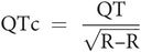
where R–R is the interval measured between two R waves.
The ST segment and T wave are associated with ventricular repolarisation. The ventricles remain contracted until a few milliseconds after repolarisation ends.
The U wave remains controversial in its origin. It may represent the slow repolarisation of the papillary muscles.
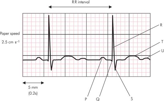
Sample electrocardiogram trace
Electrical axis of the heart
Electrical activity in the heart can be represented by a vector, since it possesses both amplitude and direction. A single or resultant vector can be drawn showing the magnitude and direction of the electrical activity in the heart at any instant. This will change continuously throughout the cardiac cycle. Thus a vector can be drawn to represent maximum electrical activity for any wave of the ECG. During the QRS complex, a maximum vector is normally produced pointing downwards and to the left. This vector reflects peak electrical activity during mass depolarisation of the ventricles, and its direction is referred to as the electrical axis of the heart or the cardiac axis. Various factors may vary the direction of this axis, including the anatomical position of the heart and different pathological conditions (e.g. left ventricular hypertrophy).
ECG leads
An electrical signal is a potential difference detected between two points. In the ECG, signals are recorded between two active surface electrodes, or an active electrode and a common or indifferent point. Each signal recorded is called a lead and may have an amplitude of several millivolts. There are 12 conventional ECG leads. They may be divided into two groups:
Frontal-plane leads:
Standard leads I, II and III
Unipolar limb leads aVR, aVL and aVF
Horizontal-plane leads:
Precordial/chest leads V1–V6
Standard limb leads I, II, III
These leads are recorded with a combination of two active electrodes at a time and are therefore bipolar leads. Each signal is recorded in the direction of the sides of an equilateral triangle with an apex on each shoulder and the pubic region, and the heart at its centre. This is called Einthoven’s triangle (Figure 14.11).
Lead I – The negative electrode is placed on the right arm and the positive electrode on the left arm.
Lead II – The negative electrode is placed on the right arm and the positive electrode on the left foot.
Lead III – The negative electrode is placed on the left arm and the positive electrode on the left foot.
The ECGs of these three leads are very similar to each other. They all record positive P waves, positive T waves and positive QRS complexes.
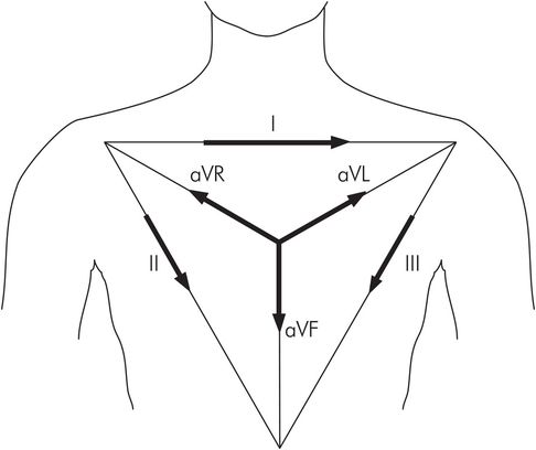
Einthoven’s triangle
Unipolar limb leads aVR, aVL, aVF
These unipolar leads record the difference between an active limb electrode and an indifferent (zero potential) electrode at the centre of Einthoven’s triangle (Figure 14.11). These signals are of lower amplitude than other leads and require increased amplification (hence referred to as augmented leads):
aVR – The augmented unipolar right arm lead faces the heart from the right side and is usually orientated to the cavity of the heart. Therefore all the deflections P, QRS and T are normally negative in this lead.
aVL – The augmented unipolar left arm lead faces the heart from the left side and is orientated to the anterolateral surface of the left ventricle.
aVF – The augmented unipolar left leg lead, orientated to the inferior surface of the heart.
Precordial chest leads
These horizontal-plane unipolar leads are placed as follows:
V1 – Fourth intercostal space immediately right of the sternum
V2 – Fourth intercostal space immediately left of the sternum
V3 – Exactly halfway between the positions of V2 and V4
V4 – Fifth intercostal space in the midclavicular line
V5 – Same horizontal level as V4 but on the anterior axillary line
V6 – Same horizontal level as V4 and V5 on the midaxillary line
Anatomical orientation of ECG electrodes
Although there is considerable variation in the position of the normal heart, the atria are usually positioned posteriorly in the chest while the ventricles form the base and anterior surface. The right ventricle is anterolateral to the left ventricle. The ventricles consist of three muscle masses. These are the free walls of the left and right ventricles and the interventricular septum. Electrical activity in the left ventricle and the interventricular septum is predominant. ECG electrodes will pick up signals from the closest structures and those producing the greatest electrical signals. Therefore ECG signals recorded from the anterior aspect of the heart are mainly due to activity in the interventricular septum, with only a small contribution from the right ventricular wall. Since ECG lead signals reflect activity in different parts of the heart because of their position, they are said to ‘look’ at different aspects of the heart:
sII, sIII and aVF look at the inferior surface of the heart.
sI and aVL are orientated towards the superior left lateral wall.
aVR and V1 face the cavity of the heart, and the deflections are mainly negative in these leads.
Leads V1 to V6 are orientated towards the anterior wall. V1 and V2 are anterior leads, V3 and V4 are septal leads, and V5 and V6 are lateral leads.
V1 and V2 examine the right ventricle, while V4 to V6 are orientated towards the septum and left ventricle.
There is no lead which is orientated directly to the posterior wall of the heart.
The heart rate in beats per minute can be determined from the ECG by measuring the time interval (in seconds) between two successive beats (R–R interval), and dividing this into 60 seconds.
Thus if R–R interval = 0.6 seconds:
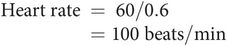
The time scale of the ECG depends on the recording paper speed. Normal paper speed is 2.5 cm s−1, meaning that each large square (5 mm) of the ECG trace represents 0.2 seconds (Figure 14.10). In the above example the R–R interval is 3 large squares (15 mm) which is equal to 0.6 seconds. If the R–R interval were to become 5 large squares (1 second) this would give a heart rate of 60 bpm.
Calculation of cardiac axis
The direction of the electrical axis of the heart is usually calculated in the frontal plane only, and can be done using two of the frontal ECG leads (these are the standard limb and unipolar limb leads). It is determined as an angle referred to the axes shown in Figure 14.12, the normal range lying between 0° and +90°.
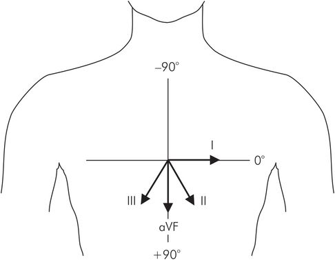
Reference axes with leads I–III and aVF
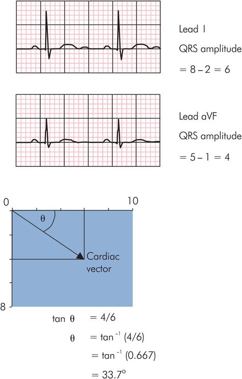
The cardiac vector, like any vector, can be resolved to give an effect or ‘component’ in any given direction. The amplitudes of the QRS complexes in the frontal leads represent components of the cardiac vector in the direction of the leads. The cardiac axis can therefore be found by the vector summation of any two of these components to find their resultant (here sI and aVF are taken for convenience since they lie at angles of 0° and 90° respectively). The direction of the cardiac axis is then given by the angle, θ, of the resultant. A simple algorithm to determine the cardiac axis from sI and aVF is presented in the green box and in Figure 14.13.
Calculation of cardiac axis
Monitoring in the operating room
During routine non-cardiac surgery sII and V5 are usually used as continuous monitoring leads. The P wave is best detected in sII, which facilitates detection of junctional or ventricular dysrhythmias. Chest lead V5 is most sensitive to ST segment changes and can warn the anaesthetist about possible ischaemia. During cardiac surgery all six of the limb leads are connected for intermittent ST segment examination, and this can increase sensitivity for the detection of ischaemia.
(shown in Figure 14.13)
Determine the amplitudes of the QRS complexes in sI and aVF by subtracting the height of the S wave from the height of the R wave in each lead.
Construct a rectangle with the sides in proportion to the amplitudes of sI and aVF. The diagonal then represents the resultant of sI and aVF (i.e. the cardiac vector).
Determine the direction of the cardiac axis from the angle θ by taking the tangent of θ as the ratio of [amplitude of aVF] / [amplitude of sI].
In practice a rapid estimation of the cardiac axis can be made simply by inspection of the frontal ECG leads. Convenient leads to use are the standard limb leads sI, sII, sIII and aVF, which lie at 0°, 60°, 120° and 90° respectively (Figure 14.12).
Initially some basic facts about the relationship between a vector and its components should be noted. The QRS amplitudes in these leads are components of the cardiac vector. The amplitude of a component depends on the angle between the component and the vector it is derived from. As this angle increases the amplitude of the component decreases.
For angles less than 90° the component is positive.
When the angle between vector and component is zero, i.e. the component is acting in the direction of the vector, the component is maximum and equal to the vector.
At 60° the amplitude of the component is half of the vector.
At 90° the amplitude of the component becomes zero.
For angles greater than 90° the component becomes negative.
Applying these simple principles confirm the following estimations:
Related posts:


Stay updated, free articles. Join our Telegram channel

Full access? Get Clinical Tree


